Simulation tests for growth rate estimators • ggoutbreak

This test data is based around a known time varying exponential growth rate with an initial epidemic seed size of 100.

Locfit models

Simple incidence test with a poisson model

An incidence mode based on absolute counts:

data = sim_poisson_model()
data %>% dplyr::glimpse()
#> Rows: 105
#> Columns: 6
#> Groups: statistic [1]
#> $ time      <time_prd> 0, 1, 2, 3, 4, 5, 6, 7, 8, 9, 10, 11, 12, 13, 14, 15, 1…
#> $ growth    <dbl> 0.1, 0.1, 0.1, 0.1, 0.1, 0.1, 0.1, 0.1, 0.1, 0.1, 0.1, 0.1, …
#> $ imports   <dbl> 100, 0, 0, 0, 0, 0, 0, 0, 0, 0, 0, 0, 0, 0, 0, 0, 0, 0, 0, 0…
#> $ rate      <dbl> 100.0000, 110.5171, 122.1403, 134.9859, 149.1825, 164.8721, …
#> $ count     <int> 97, 107, 105, 135, 148, 137, 175, 193, 239, 203, 296, 318, 3…
#> $ statistic <chr> "infections", "infections", "infections", "infections", "inf…

tmp = data %>% poisson_locfit_model(window=7, deg = 2)

plot_incidence(tmp, data)+ggplot2::geom_line(
  mapping=ggplot2::aes(x=as.Date(time),y=rate), data=data, colour="red",inherit.aes = FALSE)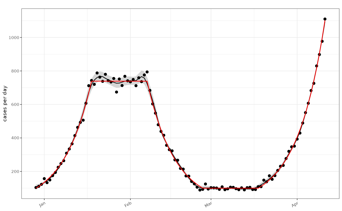

Estimated absolute growth rate versus simulation (red)


plot_growth_rate(tmp)+
  ggplot2::geom_line(mapping=ggplot2::aes(x=as.Date(time),y=growth), data=data, colour="red",inherit.aes = FALSE)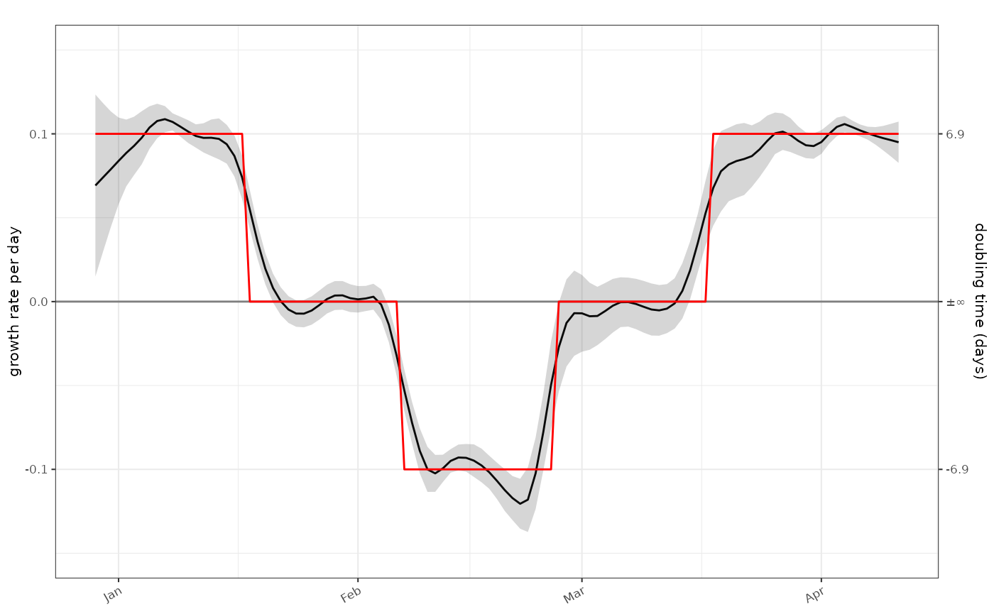


plot_growth_phase(tmp)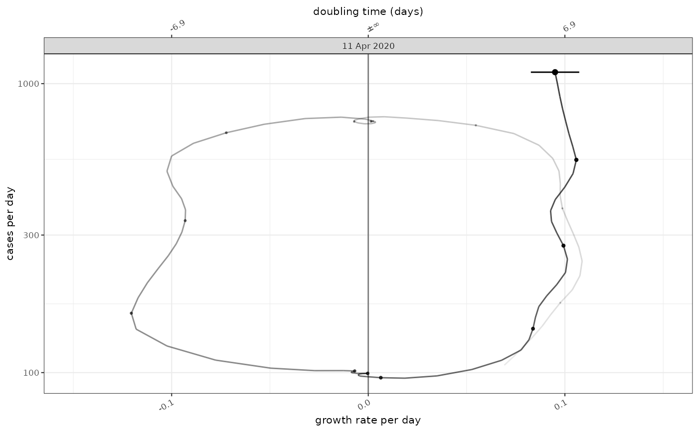

Multinomial data

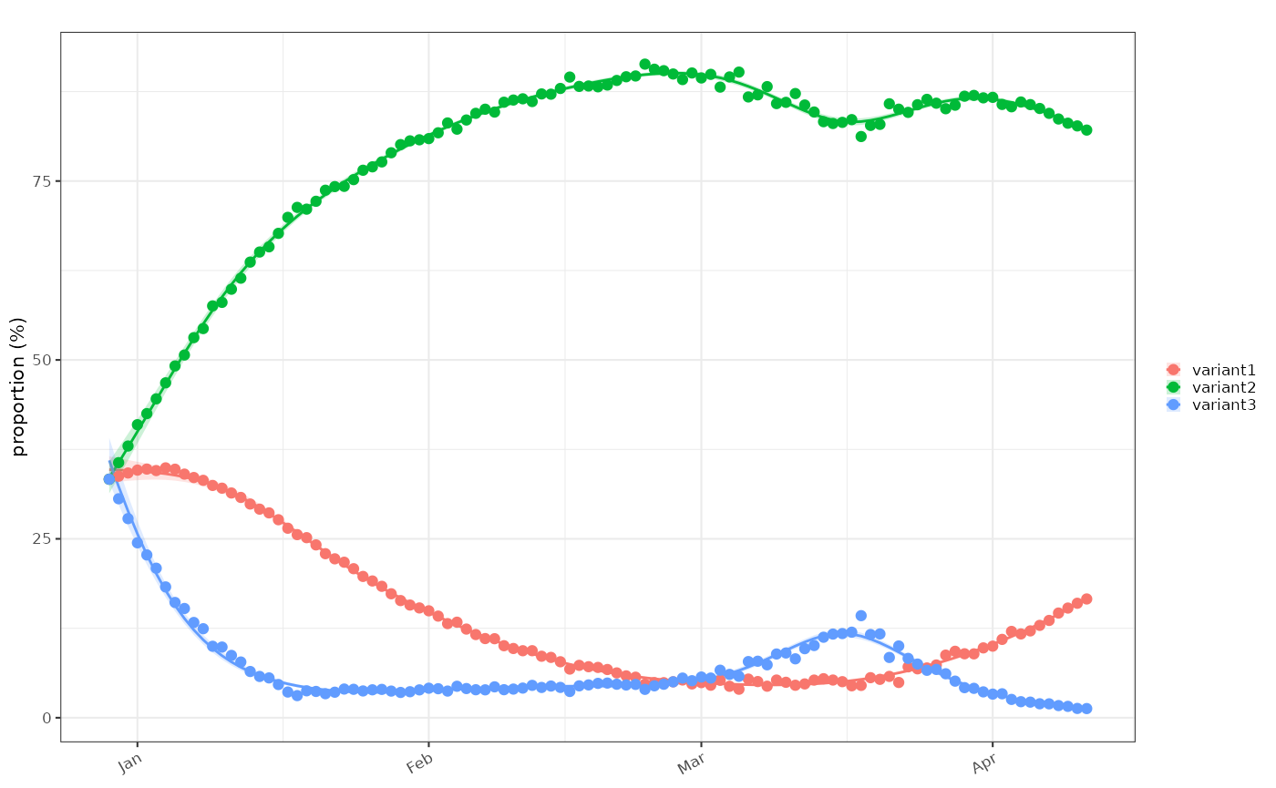
Multiple classes are simulated as 3 independent epidemics (‘variant1’, ‘variant2’ and ‘variant3’) with known growth rates and initial sample size resulting in 3 parallel time series. These are combined to give an overall epidemic and a proportional distribution of each ‘variant’ as a fraction of the whole. A relative growth rate is calculated based on set parameters.

data2 = sim_multinomial() %>% dplyr::group_by(class) %>% dplyr::glimpse()
#> Rows: 315
#> Columns: 10
#> Groups: class [3]
#> $ time            <time_prd> 0, 1, 2, 3, 4, 5, 6, 7, 8, 9, 10, 11, 12, 13, 14,…
#> $ growth          <dbl> 0.1, 0.1, 0.1, 0.1, 0.1, 0.1, 0.1, 0.1, 0.1, 0.1, 0.1,…
#> $ imports         <dbl> 100, 0, 0, 0, 0, 0, 0, 0, 0, 0, 0, 0, 0, 0, 0, 0, 0, 0…
#> $ rate            <dbl> 100.0000, 110.5171, 122.1403, 134.9859, 149.1825, 164.…
#> $ count           <int> 105, 120, 133, 141, 167, 165, 188, 182, 225, 237, 260,…
#> $ statistic       <chr> "infections", "infections", "infections", "infections"…
#> $ class           <chr> "variant1", "variant1", "variant1", "variant1", "varia…
#> $ proportion      <dbl> 0.3333333, 0.3382826, 0.3420088, 0.3445125, 0.3458146,…
#> $ proportion.obs  <dbl> 0.3333333, 0.3380282, 0.3410256, 0.3447433, 0.3457557,…
#> $ relative.growth <dbl> 0.025000000, 0.019385523, 0.013833622, 0.008404115, 0.…

Poisson model

Firstly fitting the same incidence model in a groupwise fashion:

tmp2 = data2 %>% poisson_locfit_model(window=7, deg = 1)

plot_incidence(tmp2, data2)+scale_y_log1p()

And the absolute growth rates:

plot_growth_rate(modelled = tmp2)+
   ggplot2::geom_line(mapping=ggplot2::aes(x=as.Date(time),y=growth, colour=class), data=data2, inherit.aes = FALSE)+
   ggplot2::facet_wrap(dplyr::vars(class), ncol=1)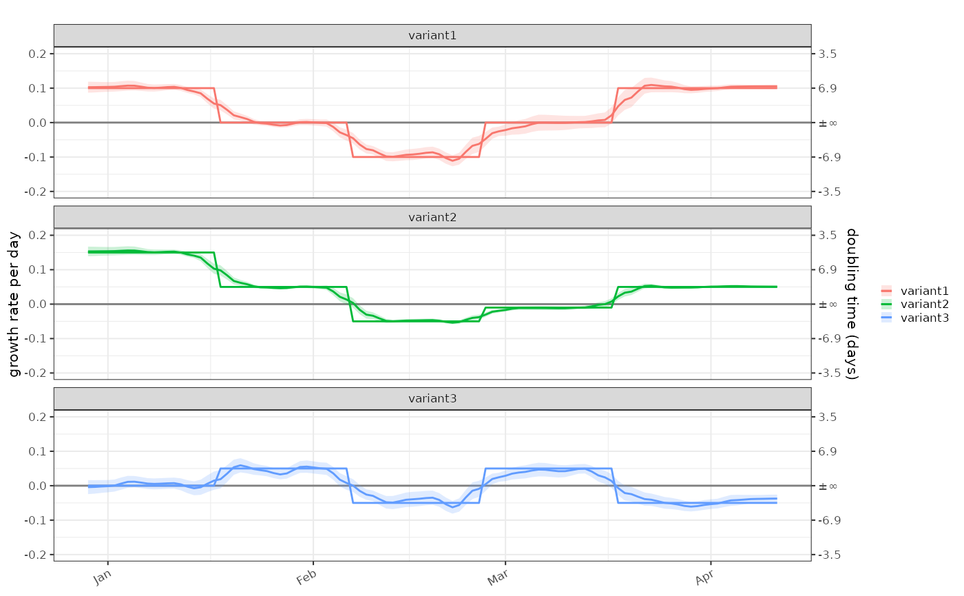

One versus others Binomial model

This looks at the proportions of the three variants and their growth rate relative to each other:

# This will reinterpret total to be the total of positives across all variants
data3 = data2 %>% 
  dplyr::group_by(time) %>% 
  dplyr::mutate(denom = sum(count)) %>%
  dplyr::group_by(class) %>%
  dplyr::glimpse()
#> Rows: 315
#> Columns: 11
#> Groups: class [3]
#> $ time            <time_prd> 0, 1, 2, 3, 4, 5, 6, 7, 8, 9, 10, 11, 12, 13, 14,…
#> $ growth          <dbl> 0.1, 0.1, 0.1, 0.1, 0.1, 0.1, 0.1, 0.1, 0.1, 0.1, 0.1,…
#> $ imports         <dbl> 100, 0, 0, 0, 0, 0, 0, 0, 0, 0, 0, 0, 0, 0, 0, 0, 0, 0…
#> $ rate            <dbl> 100.0000, 110.5171, 122.1403, 134.9859, 149.1825, 164.…
#> $ count           <int> 105, 120, 133, 141, 167, 165, 188, 182, 225, 237, 260,…
#> $ statistic       <chr> "infections", "infections", "infections", "infections"…
#> $ class           <chr> "variant1", "variant1", "variant1", "variant1", "varia…
#> $ proportion      <dbl> 0.3333333, 0.3382826, 0.3420088, 0.3445125, 0.3458146,…
#> $ proportion.obs  <dbl> 0.3333333, 0.3380282, 0.3410256, 0.3447433, 0.3457557,…
#> $ relative.growth <dbl> 0.025000000, 0.019385523, 0.013833622, 0.008404115, 0.…
#> $ denom           <int> 315, 355, 390, 409, 483, 477, 544, 531, 661, 705, 786,…

Firstly proportions:


tmp3 = data3 %>% proportion_locfit_model(window=14, deg = 2)

plot_proportion(modelled = tmp3,raw = data3)+
  ggplot2::facet_wrap(dplyr::vars(class), ncol=1)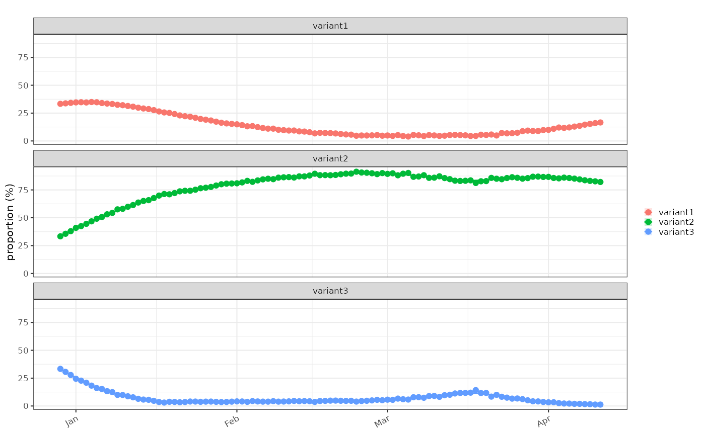

And secondly relative growth rate:



plot_growth_rate(modelled = tmp3)+
   ggplot2::geom_line(mapping=ggplot2::aes(x=as.Date(time),y=relative.growth, colour=class), data=data2, inherit.aes = FALSE)+
   ggplot2::facet_wrap(dplyr::vars(class), ncol=1)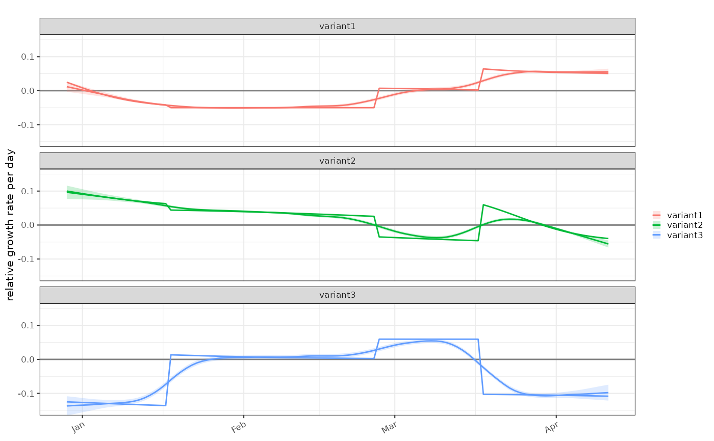


plot_growth_phase(tmp3)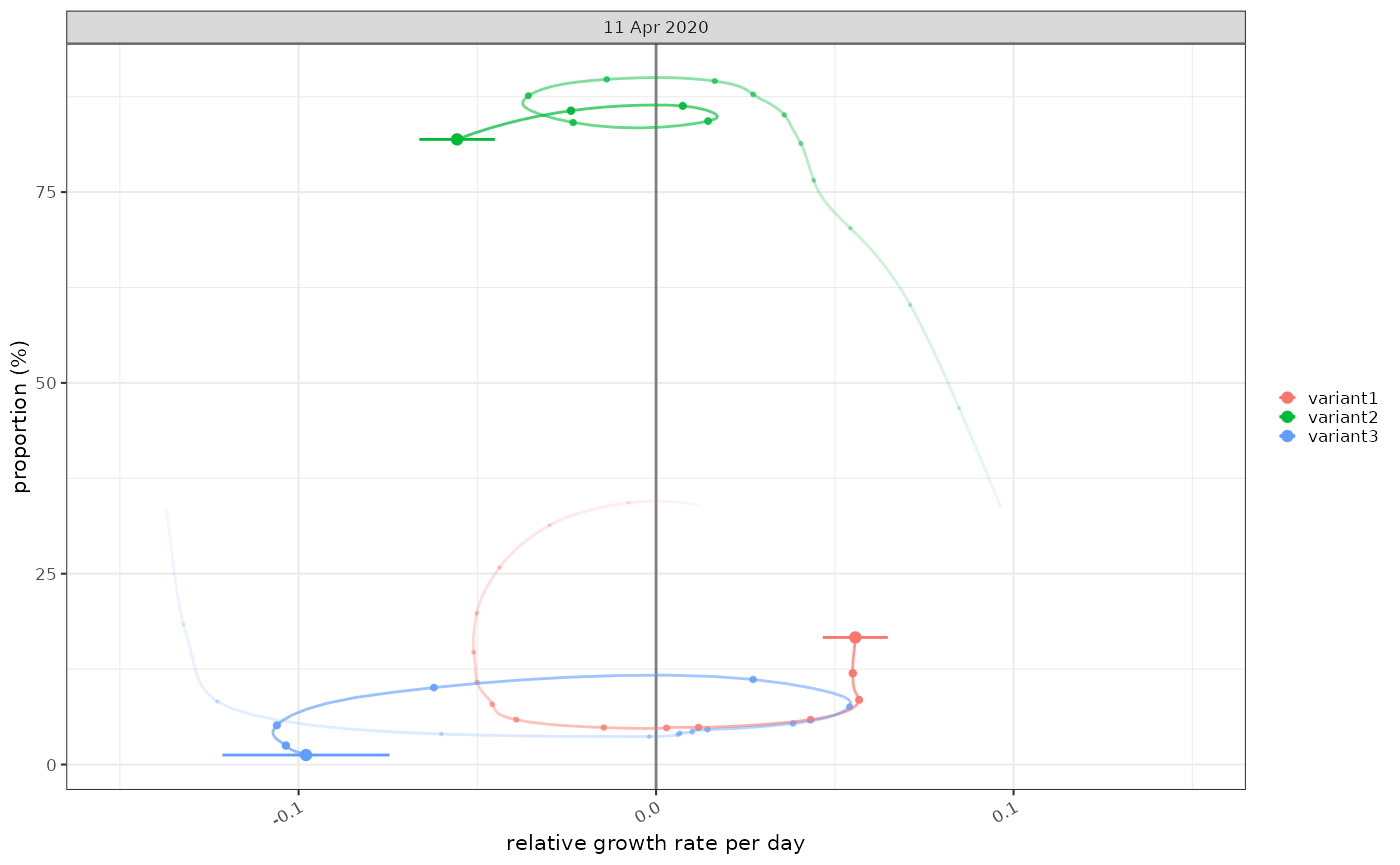

Multinomial model

The multinomial model gives us absolute proportions only (and no growth rates)

# we don't need to calculate the denominator as it is done automatically by the 
# multinomial model

tmp4 = data2 %>% multinomial_nnet_model()
#> # weights:  30 (18 variable)
#> initial  value 355342.848933 
#> iter  10 value 179670.622756
#> iter  20 value 176388.187406
#> final  value 174671.158071 
#> converged
plot_multinomial(tmp4)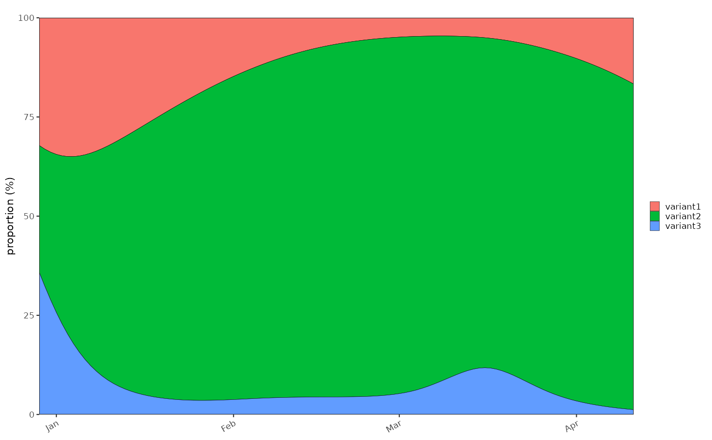


# plot_multinomial(tmp3, events = event_test,normalise = TRUE)

GLM models

Poisson model

Run a poisson model on input data using glm this returns incidence only. Derived growth rates can be estimated by using a savitsky-golay filter based approach.


tmp5 = data %>% poisson_glm_model(window=7) %>% growth_rate_from_incidence()
plot_incidence(tmp5,data)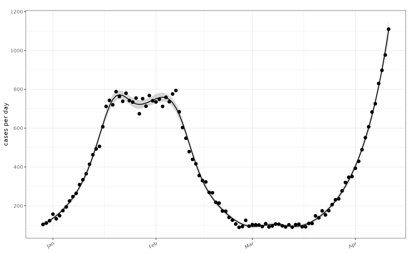


plot_growth_rate(tmp5)+
  ggplot2::geom_line(mapping=ggplot2::aes(x=as.Date(time),y=growth), data=data, colour="red",inherit.aes = FALSE)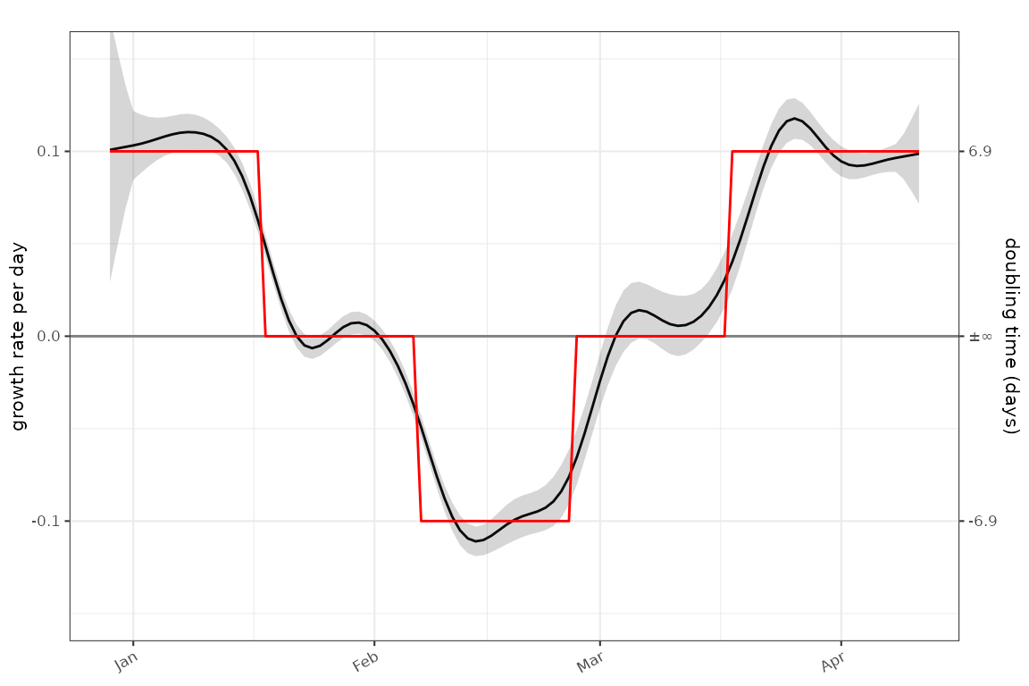


plot_growth_phase(tmp5)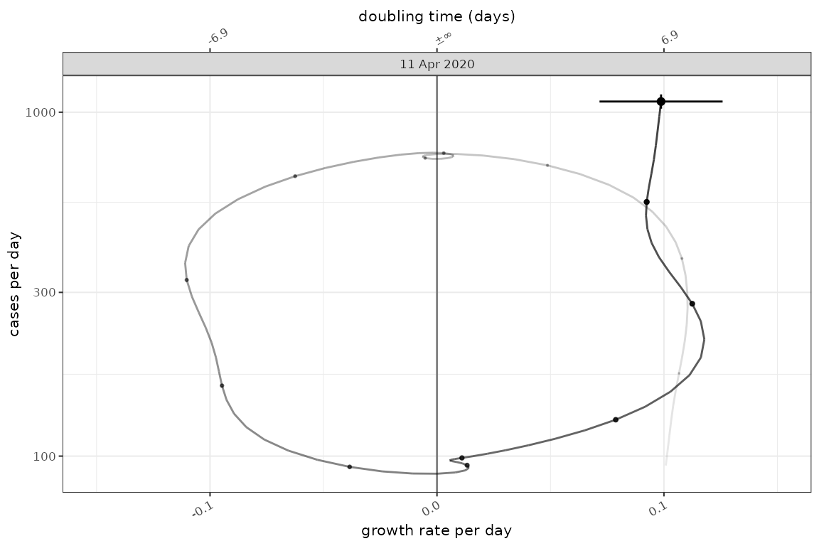

Binomial model

Run a binomial model on input data using glm this returns absolute proportions only and derived growth rates are not at this point supported.


tmp6 = data3 %>% proportion_glm_model(window=14, deg = 2)
plot_proportion(tmp6,data3)