Takes a list of times and counts and fits a quasi-poisson model
fitted with a log link function to count data using local regression
using the package locfit.
Usage
poisson_locfit_model(
  d = i_incidence_input,
  ...,
  window = 14,
  deg = 2,
  frequency = "1 day",
  predict = TRUE,
  ip = i_discrete_ip,
  quick = FALSE,
  .progress = interactive()
)
Arguments
- d
input data - a dataframe with columns:
count (positive_integer) - Positive case counts associated with the specified time frame
time (ggoutbreak::time_period + group_unique) - A (usually complete) set of singular observations per unit time as a `time_period`
Any grouping allowed.
- ...
not used and present to allow proportion model to be used in a
group_modify- window
a number of data points defining the bandwidth of the estimate, smaller values result in less smoothing, large value in more. The default value of 14 is calibrated for data provided on a daily frequency, with weekly data a lower value may be preferred. - default
14- deg
polynomial degree (min 1) - higher degree results in less smoothing, lower values result in more smoothing. A degree of 1 is fitting a linear model piece wise. - default
2- frequency
the density of the output estimates as a time period such as
7 daysor2 weeks. - default1 day- predict
result is a prediction dataframe. If false we return the
locfitmodels (advanced). - defaultTRUE- ip
An infectivity profile (optional) if not given (the default) the Rt value will not be estimated - a dataframe with columns:
boot (anything + default(1)) - a bootstrap identifier
probability (proportion) - the probability of new event during this period.
tau (integer + complete) - the days since the index event.
Minimally grouped by: boot (and other groupings allowed).
- quick
if
ipis provided, and quick isTRUERt estimation will be done assuming independence which is quicker but less accurate. Setting this to false will use a full variance-covariance matrix.- .progress
show a CLI progress bar
Value
A dataframe containing the following columns:
time (ggoutbreak::time_period + group_unique) - A (usually complete) set of singular observations per unit time as a
time_periodincidence.fit (double) - an estimate of the incidence rate on a log scale
incidence.se.fit (positive_double) - the standard error of the incidence rate estimate on a log scale
incidence.0.025 (positive_double) - lower confidence limit of the incidence rate (true scale)
incidence.0.5 (positive_double) - median estimate of the incidence rate (true scale)
incidence.0.975 (positive_double) - upper confidence limit of the incidence rate (true scale)
growth.fit (double) - an estimate of the growth rate
growth.se.fit (positive_double) - the standard error the growth rate
growth.0.025 (double) - lower confidence limit of the growth rate
growth.0.5 (double) - median estimate of the growth rate
growth.0.975 (double) - upper confidence limit of the growth rate
Any grouping allowed.
Details
This results is an incidence rate estimate plus an absolute exponential growth rate estimate both based on the time unit of the input data (e.g. for daily data the rate will be cases per day and the growth rate will be daily).
Examples
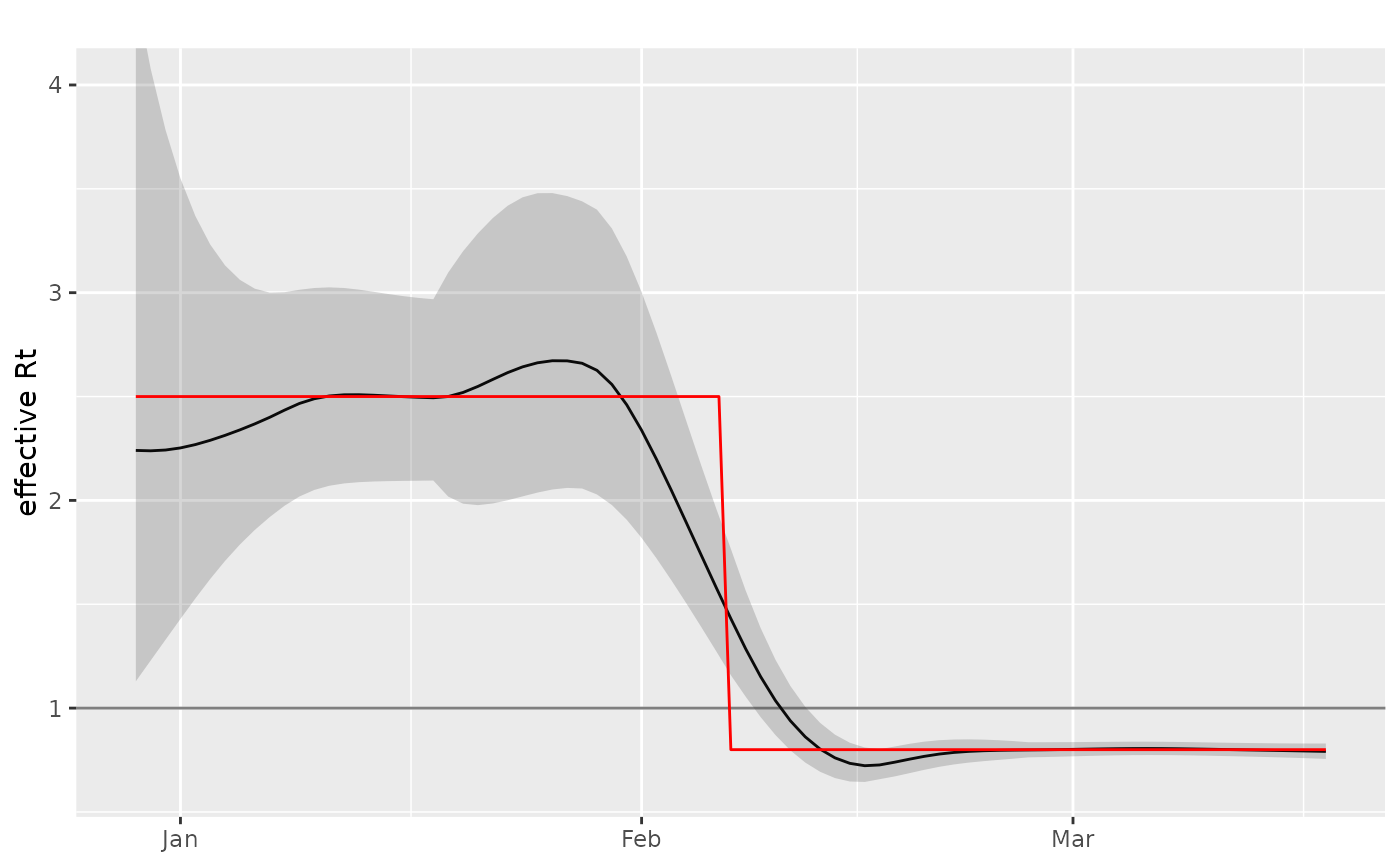
data = example_poisson_rt()
tmp = data %>% poisson_locfit_model(window=14,deg=2, ip=example_ip(), quick=TRUE)
#> Rt estimation using Locfit (approx and assuming independence)
#> Estimates were assumed to be independent, but more that 1% of estimates
#> are at risk of Rt underestimation by more that 0.05 (absolute).
#> We advise re-running supplying a full variance-covariance matrix, or
#> a value to the `raw` parameter, or setting `quick=FALSE`.
plot_rt(tmp,
    raw = data,
    true_col = rt)


data = example_poisson_growth_rate()
tmp2 = data %>% poisson_locfit_model(window=7,deg=1)
tmp3 = data %>% poisson_locfit_model(window=14,deg=2)


comp = dplyr::bind_rows(
  tmp2 %>% dplyr::mutate(class="7:1"),
  tmp3 %>% dplyr::mutate(class="14:2"),
) %>% dplyr::group_by(class)

if (interactive()) {
  plot_incidence(
    comp,
    date_labels="%b %y",
    raw=data,
    true_col = rate
  )

  plot_growth_rate(
    comp,
    date_labels="%b %y",
    raw = data,
    true_col = growth
  )
  # sim_geom_function(data,colour="black")
}
data = example_poisson_growth_rate()
tmp2 = data %>% poisson_locfit_model(window=7,deg=1)
tmp3 = data %>% poisson_locfit_model(window=14,deg=2)
comp = dplyr::bind_rows(
tmp2 %>% dplyr::mutate(class="7:1"),
tmp3 %>% dplyr::mutate(class="14:2"),
) %>% dplyr::group_by(class)
if (interactive()) {
plot_incidence(
comp,
date_labels="%b %y",
raw=data,
true_col = rate
)
plot_growth_rate(
comp,
date_labels="%b %y",
raw = data,
true_col = growth
)
# sim_geom_function(data,colour="black")
}