Estimating the reproduction number from modelled incidence

Robert Challen ^1,2; Leon Danon ^1,2;

1. Engineering Mathematics, University of Bristol, Bristol, UK
2. AI4CI

Introduction

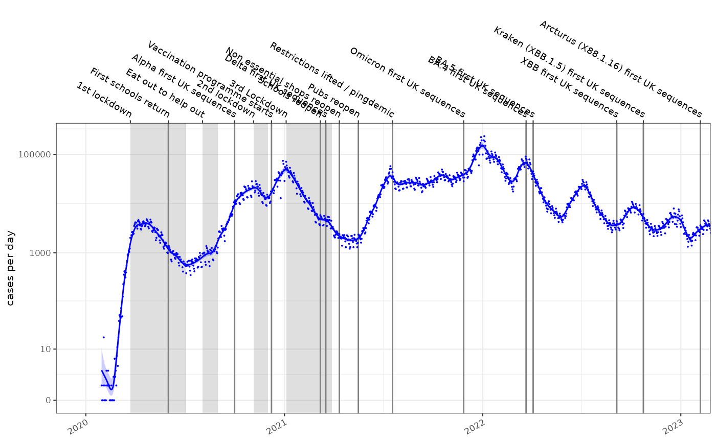
If we have estimated the incidence of a disease $I_t$ using a poisson rate using maximum likelihood estimators, the rate is typically a log-normally distributed with parameters $\mu$ and $\sigma$. Such a fitted model is shown below on a log1p scale, for the COVID-19 epidemic in England:

It is appealing to use this modelled incidence estimate to calculate an estimate of the reproduction number, $R_t$. Incidence models can be derived in a number of ways, they are easily inspected for error and can be made tolerant of missing values and outliers.

Methods

To use a modelled estimate of incidence to predict $R_t$ we need to propagate uncertainty in incidence into our $R_t$ estimates. To calculate $R_t$ we can use the backwards-looking renewal equations which incorporate the infectivity profile of the disease ($\omega$) at a number of days after infection ($\tau$):

$$\begin{eqnarray} \begin{aligned} I_t &\sim Poisson(\lambda_t) \\ \lambda_t &\sim Lognormal(\mu_t,\sigma_t) \\ R_t &= \frac{I_t}{\sum_{\tau}{\omega_{\tau}I_{t-\tau}}} \end{aligned} \end{eqnarray}$$

In expectation, this gives:

$$\begin{eqnarray} \begin{aligned} R_t &\approx \frac{\lambda_t}{\sum_{\tau=1}^{k} \omega_\tau \lambda_{t-\tau}} \\ &\sim \frac{\text{Lognormal}(\mu_t, \sigma_t)}{\sum_{\tau=1}^{k} \text{Lognormal}\left( \mu_{t-\tau} + \log \omega_\tau, \sigma_{t-\tau} \right)} \end{aligned} \tag{1} \end{eqnarray}$$

It has been shown that the sum of correlated log-normal distributed random variables can be approximated by another log-normal with parameters $\mu_Z$ and $\sigma_Z$, where the correlation between them is $\rho_{ij} = \text{Corr}(\log X_i, \log X_j)$.

$$\begin{eqnarray} \begin{aligned} S_+ &= \mathbb{E}\left[\sum_i X_i \right] = \sum_i \mathbb{E}[X_i] \\ &= \sum_i e^{\mu_i + \frac{1}{2}\sigma_i^2} \\ \sigma^2_{Z} &= \frac{1}{S_+^2} \, \sum_{i,j} \rho_{ij} \sigma_i \sigma_j \mathbb{E}[X_i] \mathbb{E}[X_j] \\ &= \frac{1}{S_+^2} \, \sum_{i,j} \rho_{ij} \sigma_i \sigma_j e^{\mu_i+\frac{1}{2}\sigma_i^2} e^{\mu_j+\frac{1}{2}\sigma_j^2} \\ \mu_Z &= \log S_+ - \frac{1}{2}\sigma_{Z}^2 \end{aligned} \tag{2} \end{eqnarray}$$

The sum term in the denominator of the renewal equation (1) consists of a set of correlated scaled log normal distributions with scale defined by the infectivity profile ($\omega$). For our case for a given time point $t$ we equate $X_i = \omega_{\tau} \lambda_{t-\tau}$, and substitute $\mu_i$ = $\mu_{t-\tau} + log(\omega_{\tau})$ and $\sigma_i = \sigma_{t-\tau}$ into (2) to account for the infectivity profile. We define $k$ to be the support of the infectivity profile ($k = |\omega|$). $m_{s}$ is the weighted contribution from incidence estimates on day $t-\tau$, and $\Sigma_{ij}$ is the covariance between log-incidence estimates from days $t-i$ and $t-j$.

$$\begin{eqnarray} \begin{aligned} m_{\tau} &= e^{\mu_{t-\tau} + \log \omega_{\tau} + \frac{1}{2}\sigma_{t-\tau}^2 } \\ \Sigma_{ij} &= \text{Cov}(\log \lambda_{t-i}, \log \lambda_{t-j}) = \rho_{(t-i)(t-j)} \sigma_{t-i} \sigma_{t-j} \\ S_{+} &= \sum_{\tau=1}^k { m_{\tau} } \\ \sigma_{Z}^2 &= \frac{ \sum_{i,j=1}^k { (m_{i} m_{j} \Sigma_{ij}) } }{S_{+}^2} \\ \mu_{Z} &= \log S_+ - \frac{1}{2}\sigma_{Z}^2 \end{aligned} \end{eqnarray}$$

With $\mu_{Z}$ and $\sigma_{Z}$ defined, $R_t$ is approximated as the ratio of two log-normals where $\Sigma_{0Z} = \text{Cov}(\log \lambda_t, \log S)$ is the covariance between the numerator and the log-denominator. Since $S = \sum_\tau X_\tau$, and using a first-order approximation, this covariance is a weighted average of the covariances between $\log \lambda_t$ and each $\log \lambda_{t-\tau}$, weighted by the relative expected contributions $m_\tau$.:

$$\begin{eqnarray} \tag{3} \begin{aligned} R_t &\sim \frac{Lognormal(\mu_t,\sigma_t)} {Lognormal( \mu_{Z}, \sigma_{Z})} \\ \mu_{R_t} &= \mu_t - \mu_{Z} = \mu_t - \log S_+ + \frac{1}{2}\sigma_{Z}^2\\ \sigma_{R_t} &= \sqrt{\sigma_t^2+\sigma_{Z}^2 - 2 \Sigma_{0Z}} \\ \Sigma_{0Z} &= \frac{\sum_{\tau=1}^k m_\tau \Sigma_{0\tau}}{\sum_{\tau=1}^k m_\tau} = \frac{1}{S_+}\sum_{\tau=1}^k m_\tau \Sigma_{0\tau}\\ R_t &\sim Lognormal(\mu_{R_t}, \sigma_{R_t}) \end{aligned} \end{eqnarray}$$

This formulation of $R_t$ from (3) assumes knowledge of the posterior or prediction covariance of the incidence estimates ($\Sigma_ij$). This is typical in modern frameworks , but in other situations may not be available. In this case we could assume the individual estimates of the incidence are independent, however this increases the uncertainty of our $R_t$ estimate and in certain circumstances introduces a potential underestimation bias, influenced by the true off-diagonal correlation mass and the certainty of the incidence estimates. An alternative approach is to assume weak stationarity and estimate a parametric correlation model from the data used to build the incidence model, using Pearson residuals to parameterise an exponential decay function based on time difference (see supporting software package for implementation). The degree of the bias is investigated further in the supplementary materials, and heuristics for assessing the significance of this bias proposed.

The method for estimating $R_t$ from modelled incidence has been described assuming a non-negative component to the infectivity profile, as it is implicit that infector and infectee are necessarily sequential in time. In the situation where symptomatic case counts are used as a proxy for incidence and the serial interval as a proxy for the infectivity profile, negative times between serial cases may be observed due to variation in delay in observation of the transmission chain. There is nothing in this framework to stop the use of a negative time for the infectivity profile, and we can directly support $R_t$ estimates in these cases.

Numerical stability

In (3) $\mu_t$ is the log-scale mean of the incidence estimate at time $t$, and $\sigma_t$ its standard deviation. These can be large, leading to numerical instability in terms involving $\exp(\mu + \sigma^2)$. However, assuming non-negative correlations and using log-space computation with optimized log-sum-exp functions , the expressions remain computationally tractable:

$$\begin{eqnarray} \begin{aligned} \log m_\tau &= \mu_{t-\tau} + \log \omega_\tau + \frac{1}{2} \sigma_{t-\tau}^2 \\ \log S_+ &= \text{logsumexp}_\tau(\log m_\tau) \\ \log \sigma_Z^2 &= \text{logsumexp}_{i,j} \left( \log m_i + \log m_j + \log \Sigma_{ij} \right) - 2 \log S_+ \\ \log \Sigma_{0Z} &= \text{logsumexp}_\tau \left( \log m_\tau + \log \Sigma_{0\tau} \right) - \log S_+ \end{aligned} \tag{4} \end{eqnarray}$$

Other relations may be implemented directly as in (3).

Infectivity profile uncertainty

This estimate of $R_t$ is conditioned on a single known infectivity profile. In reality there is also uncertainty in the infectivity profile ($\omega$) which plays a role in the definition of $\mu_{Z,t}$ and $\sigma_{Z,t}$. We cannot assume any particular distributional form for the infectivity profile, but we can use a range of empirical estimates of the infectivity profile to calculate multiple distributional estimates for $R_t$ and then combine these as a mixture distribution.

The nature of this mixture distribution will depend on the various empirical infectivity profile distributions. However, we can use general properties of mixture distributions to create estimates for the mean and variance of the reproduction number estimate ($R_t^*$) combining the uncertainty arising from multiple infection profile estimates ($\Omega$) and from the incidence estimate model itself:

$$\begin{eqnarray} \begin{aligned} E[R_t|\omega] &= e^{(\mu_{R_t,\omega} - \frac{1}{2}\sigma_{R_t,\omega}^2)} \\ V[R_t|\omega] &= \big[e^{(\sigma_{R_t,\omega}^2)} - 1\big] \big[e^{2 \mu_{R_t,\omega} + \sigma_{R_t,\omega}^2}\big] \\ E[R_t^*] &= \frac{1}{|\Omega|}\sum_{\omega \in \Omega} E[{R_t|\omega}] \\ V[R_t^*] &= \frac{1}{|\Omega|} \bigg[\sum_{\omega \in \Omega}{V[R_t|\omega]+E[R_t|\omega]^2}\bigg] - E[R_t^*]^2 \\ \end{aligned} \end{eqnarray}$$

The cumulative distribution function of the mixture is simply the arithmetic mean of the component cumulative distribution functions (conditioned on each infectivity profile). If $\Phi$ is the cumulative distribution function of the standard normal distribution:

$$\begin{eqnarray} \begin{aligned} F_{R_t^*}(x) &= \frac{1}{|\Omega|}\sum_{\omega \in \Omega}F_{R_t}(x|\omega) \\ P(R_t^* \le x) &= \frac{1}{|\Omega|}\sum_{\omega \in \Omega} P(R_{t,\omega} \le x) \\ P(R_t^* \le x) &= \frac{1}{|\Omega|}\sum_{\omega \in \Omega} \Phi\bigg(\frac{ln(x) - \mu_{R_t,\omega}}{\sigma_{R_t,\omega}}\bigg) \end{aligned} \end{eqnarray}$$

As the cumulative density function of this mixture distribution is a strictly increasing function, specific solutions for median ($q_{0.5}$) and 95% confidence intervals ($q_{0.025}$ and $q_{0.975}$) can be calculated numerically by solving the following equations:

$$\begin{eqnarray} \begin{aligned} \frac{1}{|\Omega|}\sum_{\omega \in \Omega} \Phi\bigg(\frac{ln(q_{0.025}) - \mu_{R_t,\omega}}{\sigma_{R_t,\omega}}\bigg) - 0.025 &= 0 \\ \frac{1}{|\Omega|}\sum_{\omega \in \Omega} \Phi\bigg(\frac{ln(q_{0.5}) - \mu_{R_t,\omega}}{\sigma_{R_t,\omega}}\bigg) - 0.5 &= 0 \\ \frac{1}{|\Omega|}\sum_{\omega \in \Omega} \Phi\bigg(\frac{ln(q_{0.975}) - \mu_{R_t,\omega}}{\sigma_{R_t,\omega}}\bigg) - 0.975 &= 0 \end{aligned} \end{eqnarray}$$

Numerical solutions to this are moderately expensive to perform. A reasonable approximation can be expected by matching moments of a log normal distribution to the mean $E[R_t^*]$ and variance $V[R_t^*]$ of the mixture. This gives us the final closed form estimator for the reproduction number given a set of infectivity profiles, $\overline{R_{t,\Omega}}$, as:

$$\begin{eqnarray} \begin{aligned} \mu_{t|\Omega} &= log\bigg(\frac{E[R_t^*]^2}{\sqrt{E[R_t^*]^2 + V[R_t^*]}}\bigg) \\ \sigma_{t|\Omega} &= \sqrt{log\bigg(1 + \frac{V[R_t^*]}{E[R_t^*]^2}\bigg)}\\ \overline{R_{t|\Omega}} &\sim Lognormal(\mu_{t|\Omega},\sigma_{t|\Omega}) \end{aligned} \end{eqnarray}$$

In summary we present a method for retrieving the distributional form of the reproduction number from log normally distributed probabilistic estimates of incidence arising from simple statistical count models. This includes uncertainty arising from both count models and from infectivity profile distributions. It is fully deterministic and computationally inexpensive. It does not place any particular constraints on the nature of the infectivity profile distribution and can handle distributions that have a negative component, as is sometimes seen in serial interval estimates.

Implementation

This method is implemented using the following R function, which is designed for numerical stability and speed. Generating $R_t$ estimates given modelled incidence typically occurring in a matter of seconds:

#> function (mu_t, vcov_ij = diag(sigma_t^2), omega, sigma_t = NULL, 
#>     tau_offset = 0) 
#> {
#>     omega_m = as.matrix(omega)
#>     k = nrow(omega_m)
#>     if (k != length(mu_t)) {
#>         stop("omega must have the same number of rows as length of mu_t.")
#>     }
#>     if (!all(dim(vcov_ij) == k)) {
#>         stop("vcov_ij must be a square matrix with the same dimensions as mu_t, and nrow(omega)")
#>     }
#>     omega_m = apply(omega_m, MARGIN = 2, rev)
#>     sigma_t = sqrt(diag(vcov_ij))
#>     time_Rt = length(mu_t) - tau_offset
#>     mu = mu_t[time_Rt]
#>     sigma = sigma_t[time_Rt]
#>     tmp = apply(omega_m, MARGIN = 2, function(omega) {
#>         log_m_tau = mu_t + sigma_t^2/2 + log(omega)
#>         log_S_plus = .logsumexp(log_m_tau)
#>         log_Sigma_ij = log(pmax(vcov_ij, 0))
#>         log_Sigma_0tau = log_Sigma_ij[time_Rt, ]
#>         log_sigma_Z2 = .logsumexp(outer(log_m_tau, log_m_tau, 
#>             "+") + log_Sigma_ij) - 2 * log_S_plus
#>         mu_Z = log_S_plus - 1/2 * exp(log_sigma_Z2)
#>         log_Sigma_0Z = .logsumexp(log_m_tau + log_Sigma_0tau) - 
#>             log_S_plus
#>         mu_Rt = mu - mu_Z
#>         sigma_Rt2 = sigma^2 + exp(log_sigma_Z2) - 2 * exp(log_Sigma_0Z)
#>         return(c(mu_Rt, sigma_Rt2))
#>     })
#>     mu_Rt = tmp[1, ]
#>     sigma_Rt2 = tmp[2, ]
#>     means = exp(mu_Rt + sigma_Rt2/2)
#>     vars = (exp(sigma_Rt2) - 1) * exp(2 * mu_Rt + sigma_Rt2)
#>     mean_star = mean(means)
#>     var_star = mean(vars + means^2) - mean_star^2
#>     mu_star = log(mean_star) - log(var_star/mean_star^2 + 1)/2
#>     sigma_star = sqrt(log(1 + var_star/mean_star^2))
#>     return(list(time_Rt = time_Rt, mean_Rt_star = mean_star, 
#>         var_Rt_star = var_star, meanlog_Rt_star = mu_star, sdlog_Rt_star = sigma_star, 
#>         mu_Rt_mix = mu_Rt, sigma_Rt_mix = sqrt(sigma_Rt2), quantile_Rt_fn = function(p) {
#>             .qmixlnorm(p, mu_Rt, sqrt(sigma_Rt2))
#>         }))
#> }
#> <bytecode: 0x58b456392eb0>
#> <environment: namespace:ggoutbreak>

Results

Testing this against the incidence model shown above, and comparing the results to the SPI-M-O consensus $R_t$ estimates gives us the following time-series for England. This is formally evaluated elsewhere but qualitatively is a good fit. It took a few seconds to calculate the reproduction number from this single time series with 1410 time points , which opens up the possibility of performing $R_t$ estimates in fine grained geographical or demographic subgroups.

#>    user  system elapsed 
#>  10.691   1.273  12.015

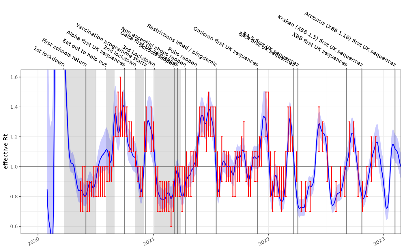
Conclusion

We present a methodology for deriving $R_t$ from modelled estimates of incidence while propagating uncertainty. We demonstrate it produces satisfactory qualitative results against COVID-19 data. This method is relatively quick, fully deterministic, and can be used on top of any statistical models for estimating incidence which use logarithmic link functions.