ggoutbreak assumes a consistent naming scheme for
significant columns, notably time and count,
and additionally class, denom,
population columns. Data needs to be supplied using these
column names and to make sure the data is formatted correctly it
undergoes quite rigorous checks. One area where this can pose problems
is in correct grouping, which must make sure that each group is a single
time series of unique time and minimally count
columns.
Line lists vs. time series
Infectious disease data usually either comes as a set of observations of an individual infection with a time stamp (i.e. a line list) or as a count of events (e.g. positive tests, hospitalisations, deaths) happening within a specific period (day, week, month etc.) as a time series.
For count data there may also be a denominator known. For testing this could be the number of tests performed, or the number of patients at risk of hospitalisation.
For both these data types there may also be a class associated with each observation, defining a subgroup of infections of interest. This could be the variant of a virus, or the age group, for example. It may make sense to compare these different subgroups against each other. In this case the denominator may be the total of counts among all groups per unit time. Additionally there may be information about the size of the population for each subgroup.
ggoutbreak assumes for the most part that the input data
is in the form of a set of time series of counts, each of which has a
unique set of times, which are usually complete. To create datasets like
this from line lists ggoutbreak provides some
infrastructure for dealing with time series
Coercing data into ggoutbreak format
A simple linelist
At the lowest level a linelist might be the list of timestamps of some observation. This is the easiest input to process and is imported into a single column data frame.
The linelist is timestamped using a S3 time_period class
which is simply a numeric of defined length time units (in this case
days) from an origin (in this case 2019-12-29). We can plot
the individual cases.
# Set the default start date and unit for `ggoutbreak`:
# This is not absolutely required as will set itself but helps in the long run
set_defaults("2019-12-29","1 day")

# Timestamps of 100 cases in first 40 days with a exponential growth rate of 0.1.
lldates = as.Date("2019-12-29")+rexpgrowth(100,0.1,40)
ll = lldates %>% linelist()
ll %>% dplyr::glimpse()
#> Rows: 100
#> Columns: 1
#> $ time <t[day]> 39.17, 22.9, 31.09, 38.32, 39.93, 33.88, 33.29, 36.65, 27.29, …
ll %>% plot_cases(individual=TRUE)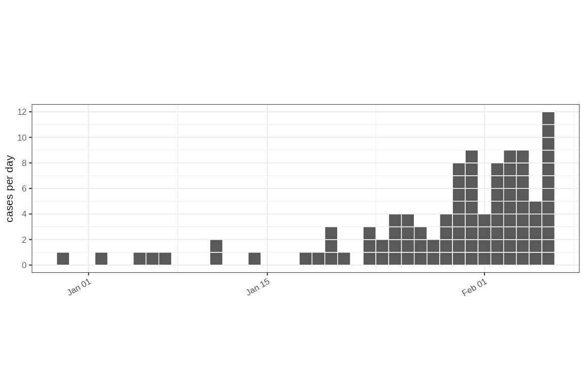
Supposing we had a slightly more complex input data. Maybe we also
had gender and age as well as a onset_dates column in a
dataframe. We can let ggoutbreak guess the structure of the
linelist, and time stamp it. If there are multiple date columns we could
also have specified the date:
lldf = dplyr::tibble(
  onset_dates = lldates,
  gender = rcategorical(100, c(male = 0.54, women = 0.46), factor = TRUE),
  age = rcategorical(100, c(`0-17` = 0.2, `18-64` = 0.6, `65+`=0.2), factor = TRUE)
)

# in this case we can let `ggoutbreak` guess the structure of this linelist:

ll2 = lldf %>% linelist()

ll2 %>% dplyr::glimpse()
#> Rows: 100
#> Columns: 4
#> $ onset_dates <date> 2020-02-06, 2020-01-20, 2020-01-29, 2020-02-05, 2020-02-0…
#> $ gender      <fct> women, women, male, male, male, women, male, women, male, …
#> $ age         <fct> 18-64, 65+, 18-64, 0-17, 0-17, 65+, 18-64, 18-64, 0-17, 65…
#> $ time        <t[day]> 39.17, 22.9, 31.09, 38.32, 39.93, 33.88, 33.29, 36.65, …

# And we can plot it with the data ordered how we like:
ll2 %>%
  dplyr::arrange(dplyr::desc(age)) %>%
  plot_cases(mapping = ggplot2::aes(fill=age), individual=TRUE)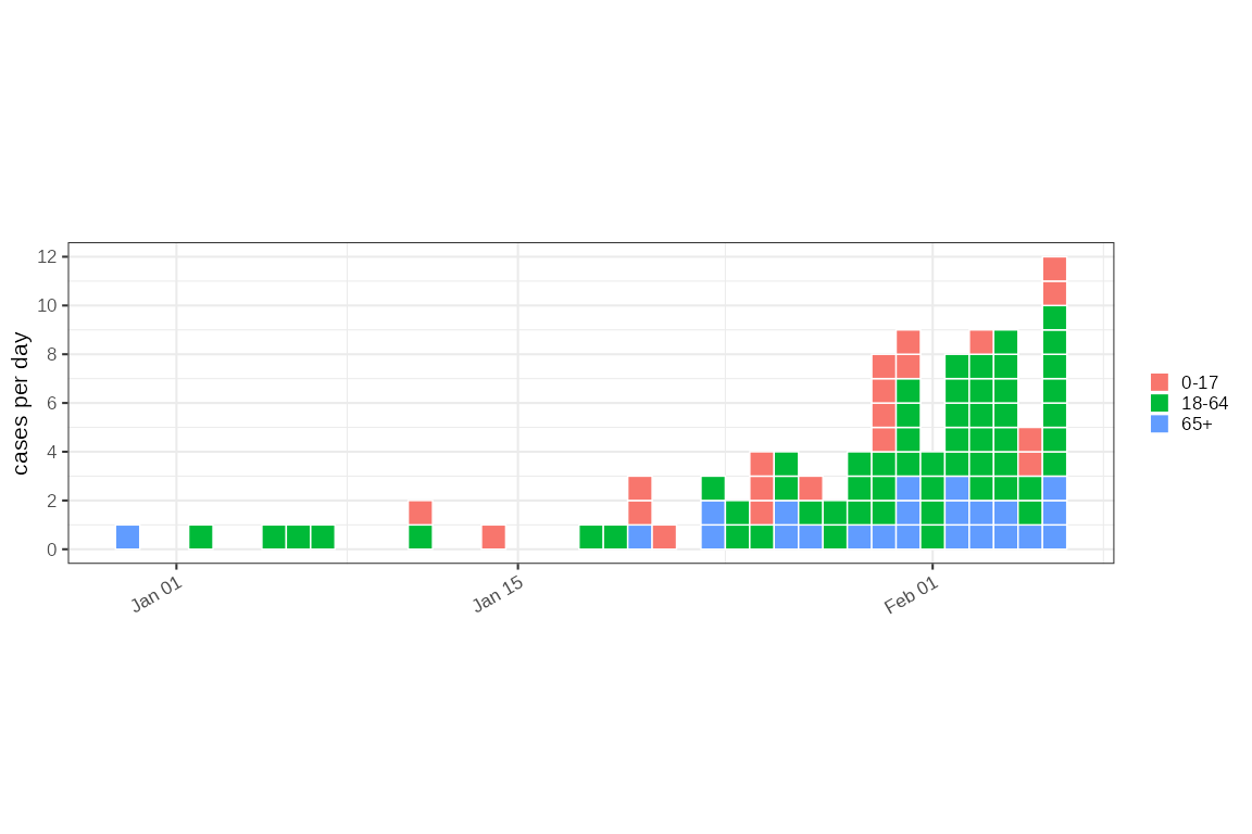
ll2 %>%
  dplyr::arrange(gender) %>%
  plot_cases(mapping = ggplot2::aes(fill=gender), individual=TRUE)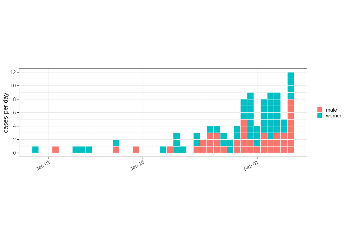
# In this case as it is a different time we can if we like anchor the time
# series to the `start` so the time column runs from zero. In this case we are
# also going to make the time stamp count in weeks:

sl2014 = outbreaks::ebola_sierraleone_2014 %>%
  linelist(date = date_of_onset, anchor="start", unit="weeks") %>%
  dplyr::mutate(
    age_cat = cut(age, c(0,18,65,Inf)),
    dplyr::across(dplyr::where(is.character),forcats::as_factor)
  ) %>%
  dplyr::glimpse()
#> Rows: 11,903
#> Columns: 10
#> $ id             <int> 1, 2, 3, 4, 5, 6, 7, 8, 9, 10, 11, 12, 13, 14, 15, 16, …
#> $ age            <dbl> 20, 42, 45, 15, 19, 55, 50, 8, 54, 57, 50, 27, 38, 29, …
#> $ sex            <fct> F, F, F, F, F, F, F, F, F, F, F, F, F, F, F, F, F, F, F…
#> $ status         <fct> confirmed, confirmed, confirmed, confirmed, confirmed, …
#> $ date_of_onset  <date> 2014-05-18, 2014-05-20, 2014-05-20, 2014-05-21, 2014-0…
#> $ date_of_sample <date> 2014-05-23, 2014-05-25, 2014-05-25, 2014-05-26, 2014-0…
#> $ district       <fct> Kailahun, Kailahun, Kailahun, Kailahun, Kailahun, Kaila…
#> $ chiefdom       <fct> Kissi Teng, Kissi Teng, Kissi Tonge, Kissi Teng, Kissi …
#> $ time           <t[week]> 0, 0.29, 0.29, 0.43, 0.43, 0.43, 0.43, 0.57, 0.57, …
#> $ age_cat        <fct> "(18,65]", "(18,65]", "(18,65]", "(0,18]", "(18,65]", "…
Plotting this is also easy, and in this case it is organised by week:
sl2014 %>%
  dplyr::arrange(status) %>%
  plot_cases(mapping = ggplot2::aes(fill=status))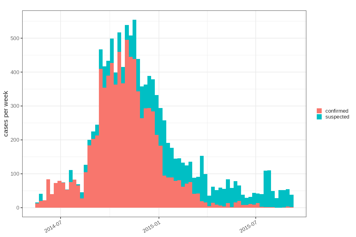
Count data
Count data describes the number of cases in a time period, e.g. a
day, a week etc. It may also be associated one or more major grouping,
such as age category, gender, geographical region, ethnicity, viral
subtype. In all these groups there is potentially a population
denominator, but often there is a major grouping that may define a
different denominator (e.g. total tested individuals). These categories
can be arbitrarily bought into ggoutbreak and managed as
groups in exactly the same was as you would in a normal
dplyr pipeline.
Because count data needs to be unique for each group for each time point extra checks are carried out to make sure that the count grouping is correct:
nhs111 = outbreaks::covid19_england_nhscalls_2020 %>%
  dplyr::group_by(sex,ccg_code,ccg_name,nhs_region) %>%
  timeseries(
    class = age
  ) %>%
  dplyr::glimpse()
#> Rows: 253,670
#> Columns: 13
#> Groups: sex, ccg_code, ccg_name, nhs_region, class, site_type [3,706]
#> $ sex        <chr> "female", "female", "female", "female", "female", "female",…
#> $ ccg_code   <chr> "e38000062", "e38000163", "e38000001", "e38000002", "e38000…
#> $ ccg_name   <chr> "nhs_gloucestershire_ccg", "nhs_south_tyneside_ccg", "nhs_a…
#> $ nhs_region <chr> "South West", "North East and Yorkshire", "North East and Y…
#> $ class      <fct> missing, missing, 0-18, 0-18, 0-18, 0-18, 0-18, 0-18, 0-18,…
#> $ time       <t[day]> 80, 80, 80, 80, 80, 80, 80, 80, 80, 80, 80, 80, 80, 80, …
#> $ site_type  <chr> "111", "111", "111", "111", "111", "111", "111", "111", "11…
#> $ date       <date> 2020-03-18, 2020-03-18, 2020-03-18, 2020-03-18, 2020-03-18…
#> $ age        <chr> "missing", "missing", "0-18", "0-18", "0-18", "0-18", "0-18…
#> $ postcode   <chr> "gl34fe", "ne325nn", "bd57jr", "tn254ab", "rm13ae", "n111np…
#> $ day        <int> 0, 0, 0, 0, 0, 0, 0, 0, 0, 0, 0, 0, 0, 0, 0, 0, 0, 0, 0, 0,…
#> $ weekday    <fct> rest_of_week, rest_of_week, rest_of_week, rest_of_week, res…
#> $ count      <int> 1, 1, 8, 7, 35, 9, 11, 19, 6, 9, 27, 13, 9, 13, 20, 6, 21, …
In this case the level of detail may be more than we want to deal with and aggregating groups maybe useful (mre details later):
nhs111combined = nhs111 %>%
  dplyr::group_by(sex,class,age) %>%
  time_aggregate() %>%
  dplyr::glimpse()
#> Rows: 1,713
#> Columns: 4
#> Groups: sex, class [12]
#> $ sex   <chr> "female", "female", "female", "female", "female", "female", "fem…
#> $ class <fct> 0-18, 0-18, 0-18, 0-18, 0-18, 0-18, 0-18, 0-18, 0-18, 0-18, 0-18…
#> $ time  <t[day]> 80, 81, 82, 83, 84, 85, 86, 87, 88, 89, 90, 91, 92, 93, 94, 9…
#> $ count <int> 10283, 10400, 9029, 8849, 9185, 9326, 7617, 6890, 5768, 5709, 58…

nhs111combined %>% plot_counts(mapping=ggplot2::aes(colour=class))+
  ggplot2::facet_wrap(~sex)+
  scale_y_log1p()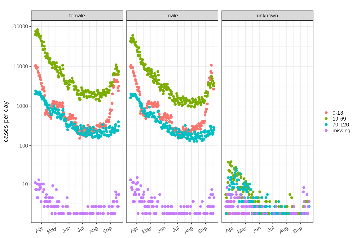
More detail on time periods
A weekly case rate represents a time slice of seven days with a start
and finish date. Dates are a continuous quantity, and
cut_dates() can be used to classify continuous dates into
periods of equal duration, with a start date:
random_dates = Sys.Date()+sample.int(21,50,replace = TRUE)
cut_date( random_dates, unit = "1 week", anchor = "start", dfmt = "%d %b")
#> 12 Dec — 18 Dec 26 Dec — 01 Jan 26 Dec — 01 Jan 19 Dec — 25 Dec 19 Dec — 25 Dec
#>    "2025-12-12"    "2025-12-26"    "2025-12-26"    "2025-12-19"    "2025-12-19"
#> 19 Dec — 25 Dec 12 Dec — 18 Dec 26 Dec — 01 Jan 26 Dec — 01 Jan 26 Dec — 01 Jan
#>    "2025-12-19"    "2025-12-12"    "2025-12-26"    "2025-12-26"    "2025-12-26"
#> 19 Dec — 25 Dec 12 Dec — 18 Dec 26 Dec — 01 Jan 19 Dec — 25 Dec 26 Dec — 01 Jan
#>    "2025-12-19"    "2025-12-12"    "2025-12-26"    "2025-12-19"    "2025-12-26"
#> 12 Dec — 18 Dec 26 Dec — 01 Jan 26 Dec — 01 Jan 12 Dec — 18 Dec 12 Dec — 18 Dec
#>    "2025-12-12"    "2025-12-26"    "2025-12-26"    "2025-12-12"    "2025-12-12"
#> 19 Dec — 25 Dec 12 Dec — 18 Dec 19 Dec — 25 Dec 26 Dec — 01 Jan 12 Dec — 18 Dec
#>    "2025-12-19"    "2025-12-12"    "2025-12-19"    "2025-12-26"    "2025-12-12"
#> 26 Dec — 01 Jan 12 Dec — 18 Dec 19 Dec — 25 Dec 26 Dec — 01 Jan 19 Dec — 25 Dec
#>    "2025-12-26"    "2025-12-12"    "2025-12-19"    "2025-12-26"    "2025-12-19"
#> 19 Dec — 25 Dec 19 Dec — 25 Dec 26 Dec — 01 Jan 26 Dec — 01 Jan 19 Dec — 25 Dec
#>    "2025-12-19"    "2025-12-19"    "2025-12-26"    "2025-12-26"    "2025-12-19"
#> 12 Dec — 18 Dec 26 Dec — 01 Jan 12 Dec — 18 Dec 19 Dec — 25 Dec 19 Dec — 25 Dec
#>    "2025-12-12"    "2025-12-26"    "2025-12-12"    "2025-12-19"    "2025-12-19"
#> 19 Dec — 25 Dec 26 Dec — 01 Jan 26 Dec — 01 Jan 12 Dec — 18 Dec 26 Dec — 01 Jan
#>    "2025-12-19"    "2025-12-26"    "2025-12-26"    "2025-12-12"    "2025-12-26"
#> 26 Dec — 01 Jan 26 Dec — 01 Jan 26 Dec — 01 Jan 26 Dec — 01 Jan 19 Dec — 25 Dec
#>    "2025-12-26"    "2025-12-26"    "2025-12-26"    "2025-12-26"    "2025-12-19"
Performing calculations using interval censored dates is awkward. A
numeric version of dates is useful that can keep track of both the start
date of a time series and its intrinsic duration, as a numeric. This is
the purpose of the time_period class:
dates = seq(as.Date("2020-01-01"),by=7,length.out = 5)
tmp = as.time_period(dates)
tmp
#> time unit: day, origin: 2019-12-29 (a Sunday)
#> 3 10 17 24 31
The time_period defaults to using the start of the first
defined time_period in a session as its origin and
calculating a duration unit based on the data (in this case weekly).
This behaviour can be controlled explicitly with
set_default_start() and set_default_unit(), or
on an ad-hoc basis by providing the start_date or
anchor and unit variables to calls to
as.time_period()
A usual set of S3 methods are available such as formatting, printing,
labelling, and casting time_periods to and from dates and
POSIXct classes:
suppressWarnings(labels(tmp))
#> [1] "01/Jan" "08/Jan" "15/Jan" "22/Jan" "29/Jan"
A weekly time series can be recast to a different frequency, or start date:
tmp2 = as.time_period(tmp, unit = "2 days", start_date = "2020-01-01")
tmp2
#> time unit: 2 days, origin: 2020-01-01 (a Wednesday)
#> 0 3.5 7 10.5 14
and the original dates should be recoverable:
as.Date(tmp2)
#> [1] "2020-01-01" "2020-01-08" "2020-01-15" "2020-01-22" "2020-01-29"
date_seq() can be used to make sure a set of periodic
times is complete:
tmp3 = as.time_period(Sys.Date()+c(0:2,4:5)*7,anchor = "start")
as.Date(date_seq(tmp3))
#> [1] "2025-12-11" "2025-12-18" "2025-12-25" "2026-01-01" "2026-01-08"
#> [6] "2026-01-15"time_periods can also be used with monthly or yearly
data but such data are not regular. This is approximately handled and
irregular date periods are generally OK to use with
ggoutbreak. Some functions like date_seq may
not work as anticipated with irregular dates, and some conversions
between weeks and months, for example, are potentially lossy.
Two time series can be aligned to make them comparable, although by default the creation of time series means they are already comparable:
orig_dates = Sys.Date()+1:10*7

# a 2 daily time series based on weekly dates
t1 = as.time_period(orig_dates, unit = "2 days", anchor = "2021-01-01")
t1
#> time unit: 2 days, origin: 2021-01-01 (a Friday)
#> 906 909.5 913 916.5 920 923.5 927 930.5 934 937.5

# a weekly with different start date
t2 = as.time_period(orig_dates, unit = "1 week", anchor = "2022-01-01")
t2
#> time unit: week, origin: 2022-01-01 (a Saturday)
#> 206.7 207.7 208.7 209.7 210.7 211.7 212.7 213.7 214.7 215.7

# rebase t1 into the same format as t2
# as t1 and t2 based on the same original dates converting t2 onto the same
# peridicty as t1 results in an identical set of times
t3 = as.time_period(t1,t2)
t3
#> time unit: week, origin: 2022-01-01 (a Saturday)
#> 206.7 207.7 208.7 209.7 210.7 211.7 212.7 213.7 214.7 215.7

# This happens automatically when the vectors are concatented
c(t1,t2)
#> time unit: 2 days, origin: 2021-01-01 (a Friday)
#> 906 909.5 913 916.5 920 923.5 927 930.5 934 937.5 906 909.5 913 916.5 920 923.5 927 930.5 934 937.5
Times in ggoutbreak and conversion of line-lists
ggoutbreak uses the time_period class
internally extensively. Casting dates to and from
time_periods is all that generally needs to be done before
using ggoutbreak and this is done automatically by
linelist() and timeseries() functions. Most of
the functions in ggoutbreak operate on time series data
which expect a unique (and usually complete) set of data on a periodic
time.
To help prepare line-list data into time series there is the
time_summarise() function. A minimal line-list will have a
date column and nothing else. From this we can generate a count of cases
over a specific time unit:
random_dates = Sys.Date()+sample.int(21,50,replace = TRUE)
linelist = dplyr::tibble(date = random_dates)
linelist %>% time_summarise(unit="1 week") %>% dplyr::glimpse()
#> Rows: 3
#> Columns: 2
#> $ time  <t[week]> 0, 1, 2
#> $ count <int> 16, 20, 14
If the line-list contains a class column it is
interpreted as a complete record of all possible options from which we
can calculate a denominator. In this case the positive and negative
results of a test:
random_dates = Sys.Date()+sample.int(21,200,replace = TRUE)
linelist2 = dplyr::tibble(
  date = random_dates,
  class = stats::rbinom(200, 1, 0.04) %>% ifelse("positive","negative")
)
linelist2 %>% time_summarise(unit="1 week") %>% dplyr::glimpse()
#> Rows: 6
#> Columns: 4
#> Groups: class [2]
#> $ class <chr> "negative", "negative", "negative", "positive", "positive", "pos…
#> $ time  <t[week]> 0, 1, 2, 0, 1, 2
#> $ count <int> 66, 76, 53, 2, 2, 1
#> $ denom <int> 68, 78, 54, 68, 78, 54
In this specific example subsequent analysis with
ggoutbreak may focus on the positive subgroup
only, as the comparison between positive and
negative test results is trivial. In another example
class may not be test results, it could be any other major
subdivision e.g. the variant of a disease. In this case the comparison
between different groups may be much more relevant. The use of
class as the major sub-group is for convenience. Additional
grouping other than class columns is also possible for
multi-faceted comparisons, and grouping is preserved but not included
automatically in the denominator, which may need to be manually
calculated:
random_dates = Sys.Date()+sample.int(21,200,replace = TRUE)
variant = apply(stats::rmultinom(200, 1, c(0.1,0.3,0.6)), MARGIN = 2, function(x) which(x==1))

linelist3 = dplyr::tibble(
  date = random_dates,
  class = c("variant1","variant2","variant3")[variant],
  gender = ifelse(stats::rbinom(200,1,0.5),"male","female")
)

count_by_gender = linelist3 %>%
  dplyr::group_by(gender) %>%
  time_summarise(unit="1 week") %>%
  dplyr::arrange(time, gender, class) %>%
  dplyr::glimpse()
#> Rows: 18
#> Columns: 5
#> Groups: gender, class [6]
#> $ gender <chr> "female", "female", "female", "male", "male", "male", "female",…
#> $ class  <chr> "variant1", "variant2", "variant3", "variant1", "variant2", "va…
#> $ time   <t[week]> 0, 0, 0, 0, 0, 0, 1, 1, 1, 1, 1, 1, 2, 2, 2, 2, 2, 2
#> $ count  <int> 2, 9, 28, 6, 10, 16, 2, 13, 22, 3, 6, 22, 2, 10, 22, 2, 10, 15
#> $ denom  <int> 39, 39, 39, 32, 32, 32, 37, 37, 37, 31, 31, 31, 34, 34, 34,…
Aggregating time series datasets.
In the case of a time series with additional grouping present,
removing a level of grouping whilst retaining time is made easier with
time_aggregate(). In this case we wish to sum
count and denom by gender, retaining the class
grouping.
count_by_gender %>%
  dplyr::group_by(class,gender) %>%
  time_aggregate() %>%
  dplyr::glimpse()
#> Rows: 9
#> Columns: 4
#> Groups: class [3]
#> $ class <chr> "variant1", "variant1", "variant1", "variant2", "variant2", "var…
#> $ time  <t[week]> 0, 1, 2, 0, 1, 2, 0, 1, 2
#> $ count <int> 8, 5, 4, 19, 19, 20, 44, 44, 37
#> $ denom <int> 71, 68, 61, 71, 68, 61, 71, 68, 61
by default time_aggregate will sum any of
count, denom and population
columns but any other behaviour can be specified by passing
dplyr::summarise style directives to the function.