Estimate relative growth rate from estimated prevalence

This assumes a prevalence that is logit-normally distributed. The exponential growth rate is the first derivative of the mu parameters of this logit-normal. On the link scale these are normally distributed. This function assumes that the time series incidence estimates are uncorrelated to estimate the error in the growth rate, which is a conservative approach resulting in more uncertainty in growth rate than might be possible through other methods. This is all based on Savitsky-Golay filters applied to the normally distributed logit-proportion estimates.

Usage

growth_rate_from_prevalence(d = i_prevalence_model, window = 7, deg = 2)

Arguments

d

a modelled proportion estimate - a dataframe with columns:

• time (ggoutbreak::time_period + group_unique) - A (usually complete) set of singular observations per unit time as a `time_period`

• prevalence.0.025 (proportion) - lower confidence limit of prevalence (true scale)

• prevalence.0.5 (proportion) - median estimate of prevalence (true scale)

• prevalence.0.975 (proportion) - upper confidence limit of prevalence (true scale)

Any grouping allowed.

window

the width of the Savitsky-Golay filter - must be odd

deg

the polynomial degree of the filter

Value

the timeseries with growth rate columns: A dataframe containing the following columns:

• time (ggoutbreak::time_period + group_unique) - A (usually complete) set of singular observations per unit time as a time_period

• proportion.fit (double) - an estimate of the proportion on a logit scale

• proportion.se.fit (positive_double) - the standard error of proportion estimate on a logit scale

• proportion.0.025 (proportion) - lower confidence limit of proportion (true scale)

• proportion.0.5 (proportion) - median estimate of proportion (true scale)

• proportion.0.975 (proportion) - upper confidence limit of proportion (true scale)

• relative.growth.fit (double) - an estimate of the relative growth rate

• relative.growth.se.fit (positive_double) - the standard error the relative growth rate

• relative.growth.0.025 (double) - lower confidence limit of the relative growth rate

• relative.growth.0.5 (double) - median estimate of the relative growth rate

• relative.growth.0.975 (double) - upper confidence limit of the relative growth rate

Any grouping allowed.

Examples

data = example_poisson_rt_2class()

tmp = data %>%
  proportion_glm_model(window=7,deg=2) %>%
  dplyr::select(time, dplyr::starts_with("proportion")) %>%
  dplyr::rename_with(~ gsub("proportion","prevalence",.x)) %>%
  dplyr::select(-prevalence.fit, -prevalence.se.fit)
#> Adding missing grouping variables: `class`

tmp = tmp %>%
  growth_rate_from_prevalence(window = 25, deg=1)

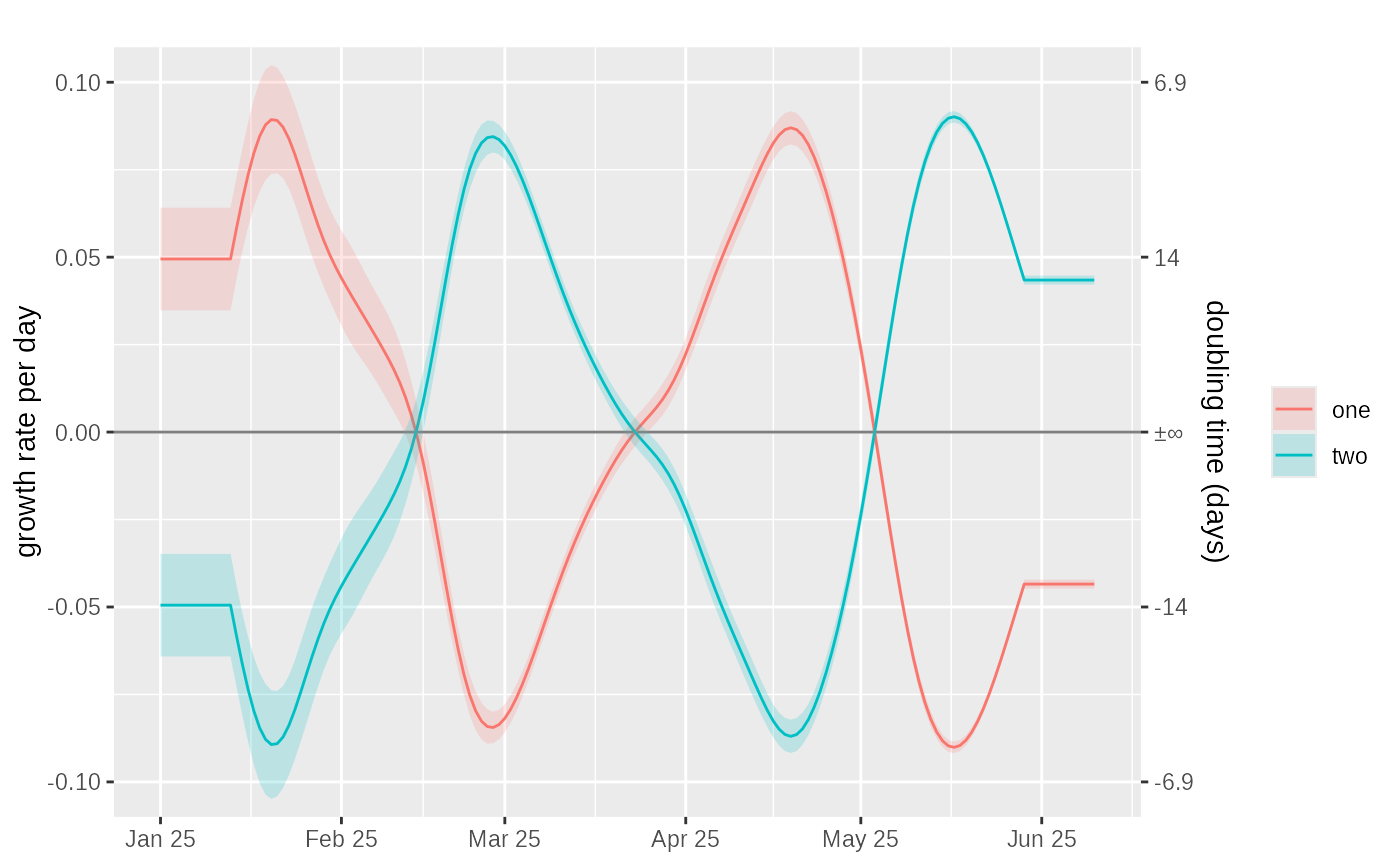
plot_growth_rate(
      tmp,
      date_labels="%b %y"
  )


data1 = ukc19::ons_infection_survey %>%
  dplyr::filter(name=="England") %>%
  timeseries(count=FALSE)

tmp2 = data1 %>%
  growth_rate_from_prevalence(window = 25, deg=1)

if(interactive()) {
  plot_growth_rate(
      tmp2,
      date_labels="%b %y",
      mapping = ggplot2::aes(colour=name),
      events = ukc19::timeline
  )
}