Fit a piecewise logit transformed linear model to weighted data
Source:R/dist-empirical.R
empirical_data.RdThis fits a CDF and quantile function to ranked data in a
transformed space. X value transformation is specified in the link
parameter and is either something like "log", "logit", etc.
Arguments
- x
either a vector of samples from a distribution
Xor cut-offs for cumulative probabilities when combined withp- w
for data fits, a vector the same length as
xgiving the importance weight of each observation. This does not need to be normalised. There must be some non zero weights, and all must be finite.- link
a link function. Either as name, or a
link_fnsS3 object. In the latter case this could be derived from a statistical distribution byas.link_fns(<dist_fns>). This supports the use of a prior to define the support of the empirical function, and is designed to prevent tail truncation. Support for the updated quantile function will be the same as the provided prior.- ...
Named arguments passed on to
.logit_z_interpolationbwa bandwidth expressed in terms of the probability width, or proportion of observations.
Named arguments passed on to
empirical_cdfsmoothfits the empirical distribution with a pair of splines for CDF and quantile function, creating a mostly smooth density. This smoothness comes at the price of potential over-fitting and will produce small differences between
pandqfunctions such thatx=p(q(x))is no longer exactly true. Setting this to false will replace this with a piecewise linear fit that is not smooth in the density, but is exact in forward and reverse transformation....not used
- name
a label for this distribution. If not given one will be generated from the distribution and parameters. This can be used as part of plotting.
- bw
a bandwidth expressed in terms of the probability width, or proportion of observations.
Value
a dist_fns S3 object that function that contains statistical
distribution functions for this data.
Details
The empirical distribution fitted is a piecewise linear in z transformed X and logit Y space. The evaluation points are linearly interpolated in this space given a bandwidth for interpolation.
Link Transformation: Input data
xis transformed using the specified link function: \(x_T = T(x)\), where \(T\) is the transformation defined by thelinkargument.Standardization (Z-space): Transformed values \(x_T\) are standardized: \(x_Z = \frac{x_T - \mu_{w,T}}{\sigma_{w,T}}\), where \(\mu_{w,T}\) and \(\sigma_{w,T}\) are the weighted mean and standard deviation of \(x_T\).
Weighted Empirical CDF: The cumulative weights are calculated to form probabilities \(y = P(X_T \leq x_T)\).
Logit Transformation: CDF probabilities are transformed: \(y_L = \text{logit}(y)\).
Local Fitting (via
.logit_z_locfit): Local likelihood models (usinglocfit) are fitted between \(x_Z\) and \(y_L\) to represent the CDF, its derivative (density), and the inverse (quantile) function in the transformed space.Function Construction: The final
p,q,r, anddfunctions are constructed by composing the fitted models from step 5 with the inverse link transformation \(T^{-1}\). For example, the final CDF is \(P(X \leq q) = F_{fitted}(\text{logit}^{-1}(T(q)))\), and the final quantile function is \(Q(p) = T^{-1}(Q_{fitted}(p))\), where \(Q_{fitted}\) is the quantile function derived from the fitted models in Z-space.
This function imputes tails of distributions. Given perfect data as samples or as quantiles it should recover the tail
Unit tests
# from samples:
withr::with_seed(123,{
 e2 = empirical_data(rnorm(10000), bw=0.1)
 testthat::expect_equal(e2$p(-5:5), pnorm(-5:5), tolerance=0.01)
 testthat::expect_equal(e2$d(-5:5), dnorm(-5:5), tolerance=0.05)
 testthat::expect_equal(e2$q(seq(0,1,0.1)), qnorm(seq(0,1,0.1)), tolerance=0.025)
})


# Construct a normal using a sequence and density as weight.
e7 = empirical_data(
  x=seq(-10,10,length.out=1000),
  w=dnorm(seq(-10,10,length.out=1000))
)
plot(e7)+ggplot2::geom_function(fun = dnorm)
testthat::expect_equal(e7$p(-5:5), pnorm(-5:5), tolerance=0.01)
Examples
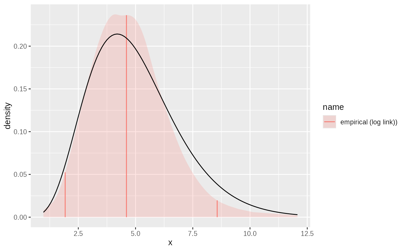
# A random sample from a distribution:
sample = rgamma2(1000, mean=5, sd=2)
# fit direct from data
fit = empirical(sample, link="log")
plot(fit)+ggplot2::geom_function(fun= ~ dgamma2(.x, mean=5, sd=2))
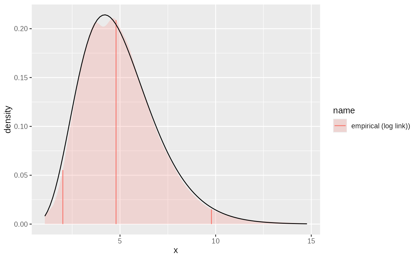 # fit weighted data
samples = seq(0,10,0.1)
weights = dgamma2(samples, mean=5, sd=2)
fit3 = empirical(x=samples, w=weights, link="log")
plot(fit3)+ggplot2::geom_function(fun= ~ dgamma2(.x, mean=5, sd=2))
# fit weighted data
samples = seq(0,10,0.1)
weights = dgamma2(samples, mean=5, sd=2)
fit3 = empirical(x=samples, w=weights, link="log")
plot(fit3)+ggplot2::geom_function(fun= ~ dgamma2(.x, mean=5, sd=2))