Getting started with tidyabc • tidyabc

library(tidyabc)
#> 
#> Attaching package: 'tidyabc'
#> The following objects are masked from 'package:base':
#> 
#>     transform, truncate
library(dplyr)
#> 
#> Attaching package: 'dplyr'
#> The following objects are masked from 'package:stats':
#> 
#>     filter, lag
#> The following objects are masked from 'package:base':
#> 
#>     intersect, setdiff, setequal, union
library(ggplot2)

ggplot2::set_theme(theme_minimal())

Introduction

This vignette walks you through a complete Approximate Bayesian Computation (ABC) workflow using tidyabc, from defining a simulation model to fitting parameters from observed data. ABC is used when the likelihood function is intractable or expensive to compute — common in complex models like those in systems biology, ecology, or social science.

We’ll simulate data from a model with two latent processes — a normal distribution and a gamma distribution — and then use ABC to recover their parameters from summary statistics, even without knowing the exact likelihood.

Step 1: Define the Simulation Function

We begin by defining a simulation function that generates synthetic data from known parameters. This represents our “forward model” — the mechanism we believe generated the real-world observations.

# example simulation
# We'll be trying to recover norm and gamma parameters
# We'll use this function for both example generation and fitting
test_simulation_fn = function(norm_mean, norm_sd, gamma_mean, gamma_sd) {
  
  A = rnorm(1000, norm_mean, norm_sd)
  B = rgamma2(1000, gamma_mean, gamma_sd)
  C = rgamma2(1000, gamma_mean, gamma_sd)

  return(
    list(
      data1 = A + B - C,
      data2 = B * C
    )
  )
  
}

Here, data1 = A + B - C combines a normal variable with two gamma variables, and data2 = B * C is their product. The true parameters are unknown to the ABC algorithm — we’ll recover them from summary statistics.

Step 2: Define the Scoring Function

Since we can’t compute the likelihood directly, we compare simulated and observed data using summary statistics. Here, we use the Wasserstein distance — a robust metric for comparing distributions — to measure how similar the simulated and observed data are for each output.

test_scorer_fn = function(simdata, obsdata) {
  return(list(
    data1 = calculate_wasserstein(simdata$data1, obsdata$data1),
    data2 = calculate_wasserstein(simdata$data2, obsdata$data2)
  ))
}

Each element of the returned list represents a distance between the simulated and observed version of data1 and data2. These distances become the basis for accepting or rejecting parameter proposals.

Step 3: Generate Observed Data (Ground Truth)

We now generate “observed” data using known parameters — this simulates real-world measurements. In practice, this would come from your actual dataset.

tmp = test_simulation(
  test_simulation_fn,
  test_scorer_fn,
  norm_mean = 4, norm_sd=2, gamma_mean=6, gamma_sd=2,
  seed = 123
)

truth = tmp$truth
test_obsdata = tmp$obsdata

The test_simulation() function runs the model once with the specified parameters and returns both the raw simulated data (obsdata) and the summary distances (obsscores). The truth object contains the known parameter values:
- norm_mean = 4
- norm_sd = 2
- gamma_mean = 6
- gamma_sd = 2

We’ll see how well ABC recovers these values.

Step 4: Visualize the Observed Data

Let’s look at the two summary variables we’re using for inference.

ggplot(
  tibble(data1 = test_obsdata$data1), aes(x=data1))+
  geom_histogram(bins=50, fill="steelblue", color="white")+
  xlab("A + B - C")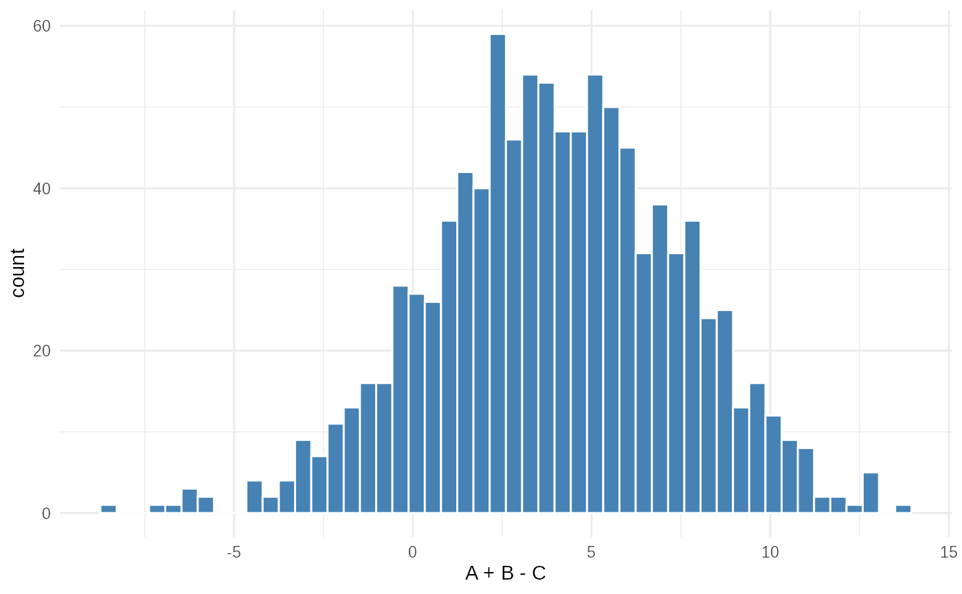


ggplot(tibble(data2 = test_obsdata$data2), aes(x=data2))+
  geom_histogram(bins=50, fill="coral", color="white")+
  xlab("B × C")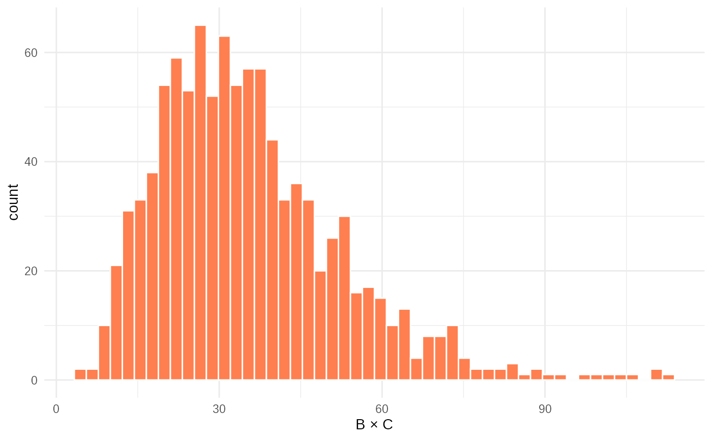

These histograms show the empirical distributions of the two summary statistics. data1 is roughly symmetric (due to the normal + gamma combination), while data2 is right-skewed (product of two gamma variables). ABC will use these shapes to infer the underlying parameters.

Step 5: Define Prior Distributions

In Bayesian inference, we express our uncertainty about the parameters before seeing the data using priors. Here, we define uniform priors for all parameters, and add a constraint to ensure the gamma distribution has a meaningful shape (mean > standard deviation).

test_priors = priors(
  norm_mean ~ unif(0, 10),
  norm_sd ~ unif(0, 10),
  gamma_mean ~ unif(0, 10),
  gamma_sd ~ unif(0, 10),
  # enforces convex gamma: mean > sd
  ~ gamma_mean > gamma_sd 
)

test_priors
#> Parameters: 
#> * norm_mean: unif(min = 0, max = 10)
#> * norm_sd: unif(min = 0, max = 10)
#> * gamma_mean: unif(min = 0, max = 10)
#> * gamma_sd: unif(min = 0, max = 10)
#> Constraints:
#> * gamma_mean > gamma_sd

The output shows the prior distributions for each parameter and the constraint. The constraint ~ gamma_mean > gamma_sd ensures that the gamma distribution is not overly flat — a common real-world assumption.

Step 6: Run ABC Rejection Sampling

Now we perform ABC rejection sampling: generate many parameter sets from the prior, simulate data for each, and accept those whose summary statistics are close enough to the observed ones.

rejection_fit = abc_rejection(
  obsdata = test_obsdata,
  priors_list = test_priors,
  sim_fn = test_simulation_fn,
  scorer_fn = test_scorer_fn,
  n_sims = 10000,
  acceptance_rate = 0.01,
  parallel = FALSE
)
#> ABC rejection, 1 wave.

summary(rejection_fit)
#> ABC rejection fit: single wave
#> Parameter estimates:
#> # A tibble: 4 × 4
#> # Groups:   param [4]
#>   param      mean_sd       median_95_CrI           ESS
#>   <chr>      <chr>         <chr>                 <dbl>
#> 1 gamma_mean 5.956 ± 0.360 5.965 [5.103 — 6.729]  78.7
#> 2 gamma_sd   2.010 ± 0.640 2.106 [0.599 — 3.307]  78.7
#> 3 norm_mean  3.863 ± 0.832 3.835 [2.093 — 6.050]  78.7
#> 4 norm_sd    2.314 ± 1.282 2.208 [0.166 — 4.935]  78.7

n_sims = 10000: We simulate 10,000 parameter sets.
acceptance_rate = 0.01: We accept the top 1% of simulations with smallest distances (i.e., best matches).

The summary() output shows: - The median and IQR of the posterior for each parameter (i.e., the best estimates after conditioning on the data). - The Effective Sample Size (ESS): a measure of how much information is in the posterior (higher = better). - The convergence status.

Compare the posterior medians to the true values (truth). With enough simulations and a good distance metric, we expect them to be close.

Step 7: Plot the Results

Finally, we visualize the posterior distributions alongside the true parameter values.

plot(rejection_fit, truth=truth)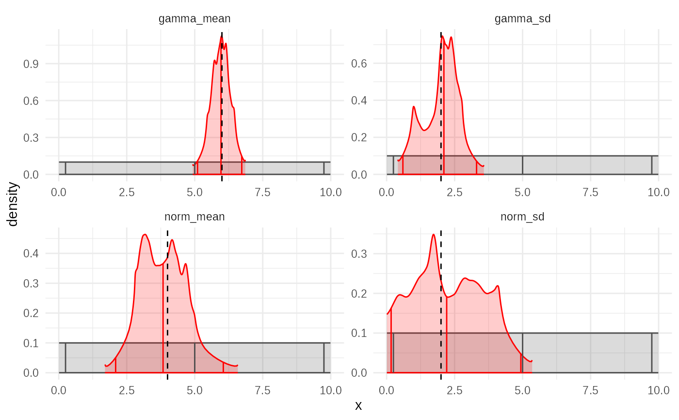

The plot shows: - Marginal posterior densities for each parameter (red curves), estimated using empirical distribution fitting. - Dotted vertical lines indicating the true parameter values (truth). - Solid vertical marks representing the median and 95% credible intervals.

If the true values lie within the credible intervals and are near the peak of the posterior, we can conclude that ABC successfully recovered the underlying parameters — even without knowing the likelihood!

Conclusion

This vignette demonstrates a complete ABC workflow that could work with observed data:

Define a simulation model (sim_fn),
Define a distance metric (scorer_fn),
Specify priors,
Run ABC rejection sampling,
Summarize and visualize the posterior.

The tidyabc package makes this process intuitive and modular. You can now replace test_simulation_fn and test_scorer_fn with your own model and summary statistics — and let ABC do the inference for you.

For more efficiency, consider switching to abc_smc() or abc_adaptive() in larger problems, which use sequential refinement to reduce the number of required simulations.