Fit a piecewise logit transformed linear model to cumulative data
Source:R/dist-empirical.R
empirical.RdThis creates statistical distribution functions fitting to data in a
transformed space. Inputs can either be weighted data observations (x,w pairs)
of a CDF (x,p pairs). X axis transformation is specified in the link
parameter and is either something like "log", "logit", etc or can also be
specified as a statistical distribution, or even a length 2 numeric vector
defining support.
Usage
empirical(
  x,
  ...,
  w = NULL,
  p = NULL,
  link = "ident",
  fit_spline = !is.null(knots),
  knots = NULL,
  name = NULL
)
Arguments
- x
either a vector of samples from a distribution
Xor cut-offs for cumulative probabilities when combined withp- ...
Named arguments passed on to
.logit_z_interpolationbwa bandwidth expressed in terms of the probability width, or proportion of observations.
Named arguments passed on to
empirical_cdfsmoothfits the empirical distribution with a pair of splines for CDF and quantile function, creating a mostly smooth density. This smoothness comes at the price of potential over-fitting and will produce small differences between
pandqfunctions such thatx=p(q(x))is no longer exactly true. Setting this to false will replace this with a piecewise linear fit that is not smooth in the density, but is exact in forward and reverse transformation....not used
- w
for data fits, a vector the same length as
xgiving the importance weight of each observation. This does not need to be normalised. There must be some non zero weights, and all must be finite.- p
for CDF fits, a vector the same length as
xgivingP(X <= x).- link
a link function. Either as name, or a
link_fnsS3 object. In the latter case this could be derived from a statistical distribution byas.link_fns(<dist_fns>). This supports the use of a prior to define the support of the empirical function, and is designed to prevent tail truncation. Support for the updated quantile function will be the same as the provided prior.- fit_spline
for distributions from data should we fit a spline to reduce memory usage and speed up sampling? If
knotsis given this is assumed to be true, set this to TRUE to allow knots to be determined by the data.- knots
for spline fitting from data how many points do we use to model the cdf? By default this will be estimated from the data. I recommend an uneven number, without a lot of data this will tend to overfit 9 knots for 1000 samples seems OK, max 7 for 250, 5 for 100. Less is usually more.
- name
a label for this distribution. If not given one will be generated from the distribution and parameters. This can be used as part of plotting.
Value
a dist_fns S3 object containing functions p() for CDF, q()
for quantile, and r() for a RNG, and d() for density. The density
function may be discontinuous.
Details
If the empirical distribution if from data it is fully transformed to a
logit-z space where the cumulative weighted data is interpolated with a
kernel weighted linear model.
In the case of CDF data the empirical distribution is fitted with a piecewise
linear or monotonically increasing spline fit to data in Q-Q space. The
spline is bounded by 0 and 1 in both dimensions.
This function imputes tails of distributions within the constraints of the link functions. Given perfect data as samples or as quantiles it should well approximate the tail.
If p is provided, data is treated as CDF points \((x_i, p_i)\).
The function calls empirical_cdf(x, p, ...) internally. This involves:
Transformation: \(x\) values are mapped via a link function \(T\) to a standardized scale \(q_x = T(x)\).
Interpolation: Monotonic splines (or piecewise linear functions if
smooth=FALSE) are fitted between \((q_x, p)\) pairs in Q-Q space, yielding functions \(F_{cdf}(q_x)\) and \(F_{qf}(p)\).Tail Extrapolation: The fit is extended to \((0,0)\) and \((1,1)\) if necessary.
Final Functions: \(P(X \leq x) = F_{cdf}(T(x))\) and \(Q(p) = T^{-1}(F_{qf}(p))\).
If w is provided (or p is NULL), data is treated as weighted samples \((x_i, w_i)\).
The function calls empirical_data(x, w, ...) internally. This involves:
Transformation: \(x\) values are mapped via a link function \(T\) to \(x_T = T(x)\).
Standardization: Values are standardized \(x_Z = (x_T - \mu_{w,T})/\sigma_{w,T}\).
Weighted CDF: Empirical CDF \(y = P(X_T \leq x_T)\) is calculated from \(w\).
Logit Transformation: \(y_L = \text{logit}(y)\).
Local Fitting:
locfitis used to fit models between \(x_Z\) and \(y_L\).Final Functions: Composed from fitted models and the inverse link \(T^{-1}\).
If fit_spline=TRUE (or knots is specified) when fitting from data,
the resulting empirical_data fit is re-interpolated using empirical_cdf
at quantiles defined by knots.
Unit tests
# from samples:
withr::with_seed(123,{
 e2 = empirical(rnorm(10000))
 testthat::expect_equal(e2$p(-5:5), pnorm(-5:5), tolerance=0.01)
 testthat::expect_equal(e2$q(seq(0,1,0.1)), qnorm(seq(0,1,0.1)), tolerance=0.05)
})

p2 = seq(0,1,0.1)
testthat::expect_equal( e2$p(e2$q(p2)), p2, tolerance = 0.001)

# updating a prior, with a horribly skewed gamma distribution
# not a great fit but not great data
withr::with_seed(124,{
  data = rgamma(500,1)
  e4 = empirical(data, link=as.dist_fns("unif",0,10))
  if (interactive()) plot(e4)+ggplot2::geom_function(fun = ~ dgamma(.x, 1))
  testthat::expect_equal(mean(e4$r(10000)), 1, tolerance=0.1)

  e5 = empirical(data,link="log")
  testthat::expect_equal(mean(e5$r(10000)), 1, tolerance=0.1)
  if (interactive()) plot(e5)+ggplot2::geom_function(fun = ~ dgamma(.x, 1))
})

withr::with_seed(123,{
  data = c(rnorm(200,4),rnorm(200,7))
  weights = c(rep(0.1,200), rep(0.3,200))
  e6 = empirical(x=data,w = weights)
  plot(e6)
  testthat::expect_equal(
    format(e6),
    "empirical; Median (IQR) 6.57 [5.2 — 7.43]"
  )
})

# Construct a normal using a sequence and density as weight.
e7 = empirical(x=seq(-10,10,length.out=1000),w=dnorm(seq(-10,10,length.out=1000)),knots = 20)
testthat::expect_equal(e7$p(-5:5), pnorm(-5:5), tolerance=0.01)
Examples
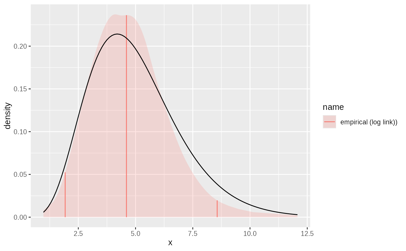
# A random sample from a distribution:
sample = rgamma2(1000, mean=5, sd=2)
# fit direct from data
fit = empirical(sample, link="log")
plot(fit)+ggplot2::geom_function(fun= ~ dgamma2(.x, mean=5, sd=2))
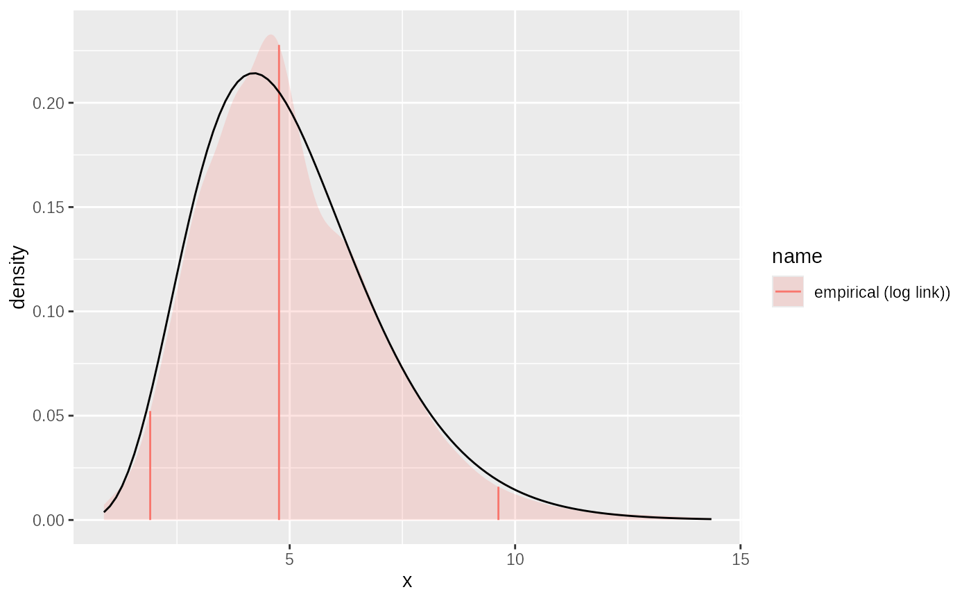 # suppose we only have quantiles
p = seq(0.1,0.9, 0.1)
quantiles = quantile(sample, p)
# fit from quantiles:
fit2 = empirical(x=quantiles,p=p, link="log")
plot(fit2)+ggplot2::geom_function(fun= ~ dgamma2(.x, mean=5, sd=2))
# suppose we only have quantiles
p = seq(0.1,0.9, 0.1)
quantiles = quantile(sample, p)
# fit from quantiles:
fit2 = empirical(x=quantiles,p=p, link="log")
plot(fit2)+ggplot2::geom_function(fun= ~ dgamma2(.x, mean=5, sd=2))
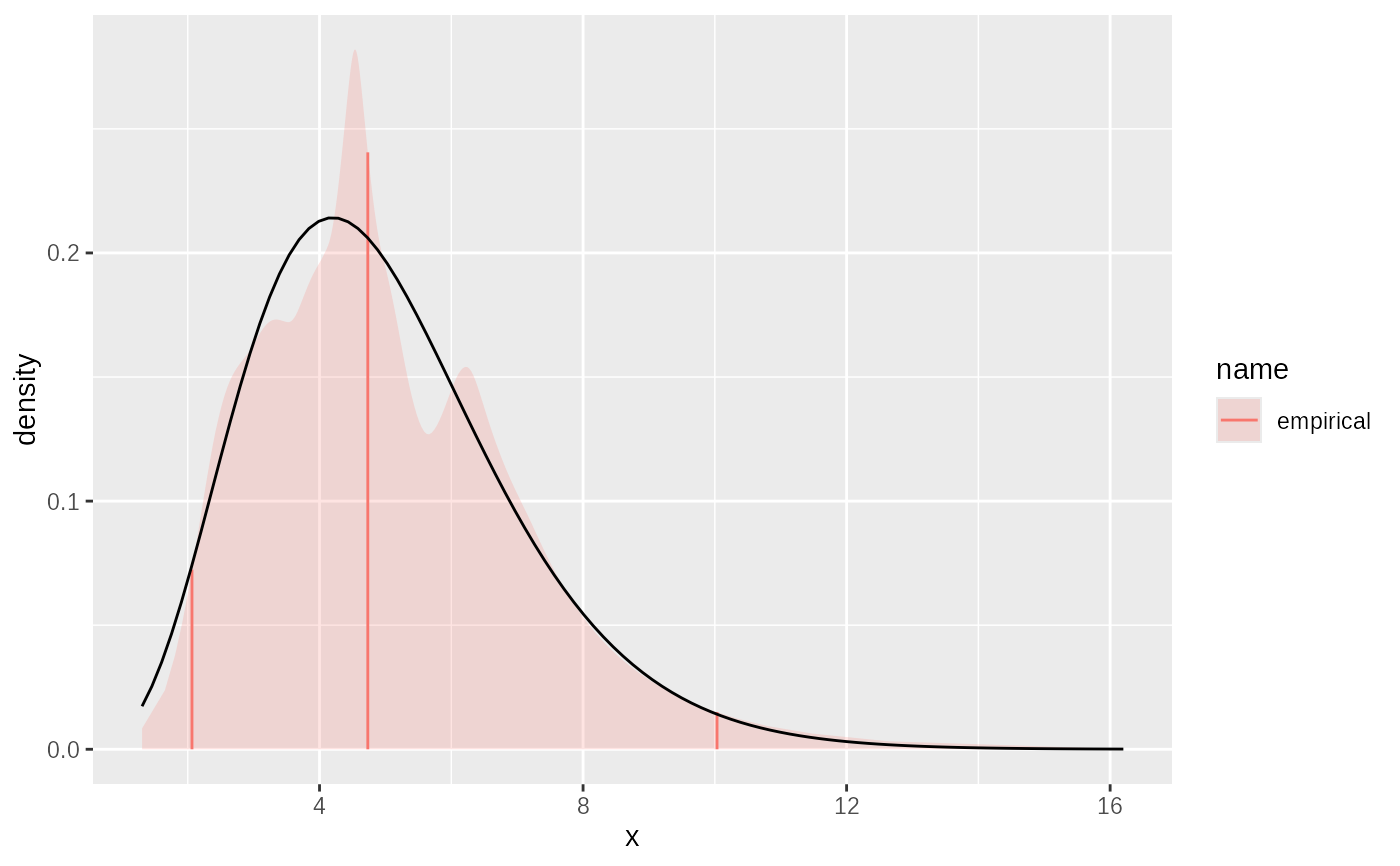 # fit weighted data
samples = seq(0,10,0.1)
weights = dgamma2(samples, mean=5, sd=2)
fit3 = empirical(x=samples, w=weights, link="log")
plot(fit3)+ggplot2::geom_function(fun= ~ dgamma2(.x, mean=5, sd=2))
# fit weighted data
samples = seq(0,10,0.1)
weights = dgamma2(samples, mean=5, sd=2)
fit3 = empirical(x=samples, w=weights, link="log")
plot(fit3)+ggplot2::geom_function(fun= ~ dgamma2(.x, mean=5, sd=2))