Generate a distribution from a truncation of another

Generates a truncated distribution from an existing distribution dist. The new distribution is restricted to the interval $[x_{left}, x_{right}]$ (or $(x_{left}, x_{right})$ if open bounds are intended, though the quantile function will map 0 to $x_{left}$ and 1 to $x_{right}$). The probability density function (PDF) of the truncated distribution $f_T(x)$ is related to the original PDF $f(x)$ by a normalization constant: $$ f_T(x) = \frac{f(x)}{F(x_{right}) - F(x_{left})} \mathbb{I}_{[x_{left}, x_{right}]}(x) $$ where $F$ is the original CDF and $\mathbb{I}$ is the indicator function. Consequently, the CDF $F_T$ and quantile function $Q_T$ are: $$ F_T(x) = \frac{F(x) - F(x_{left})}{F(x_{right}) - F(x_{left})} $$ $$ Q_T(p) = Q(F(x_{left}) + p \cdot (F(x_{right}) - F(x_{left}))) $$ where $Q$ is the quantile function of the original distribution. This function implements these transformations for the p, q, and r functions of the resulting dist_fns object.

Usage

truncate(dist, x_left, x_right, ..., name = NULL)

Arguments

dist: a distribution as a name, function or a dist_fn S3 object
x_left: The lower end of the interval or NA for open
x_right: The upper end of the interval or NA for open
...: parameters for the underlying distribution if dist is a name or function.
name: a name for the truncation

Value

a dist_fn or dist_fn_list holding the truncated distribution(s)

Unit tests




shape2_gamma = as.dist_fns(pgamma, shape=2)
g2 = truncate(shape2_gamma, 0.5, 4)

testthat::expect_equal(
  format(g2),
  "trunc(gamma(shape = 2, rate = 1), 0.50 - 4.00); Median (IQR) 1.68 [1.08 — 2.46]"
)

testthat::expect_equal(
  g2$p(0:5),
  c(0, 0.212702667019627, 0.615716430100344, 0.868531239886668, 1, 1)
)

testthat::expect_equal(g2$q(seq(0, 1, 0.2)), c(
  0.5,
  0.971743593113941,
  1.42711359317907,
  1.95304152540128,
  2.6642447272259,
  4
))


g3 = truncate(shape2_gamma, NA, 4)
testthat::expect_equal(
  format(g3),
  "trunc(gamma(shape = 2, rate = 1), 0.00 - 4.00); Median (IQR) 1.54 [0.899 — 2.35]"
)

g4 = truncate(shape2_gamma, 2, NA)
testthat::expect_equal(
  format(g4),
  "trunc(gamma(shape = 2, rate = 1), 2.00 - Inf); Median (IQR) 2.97 [2.42 — 3.87]"
)

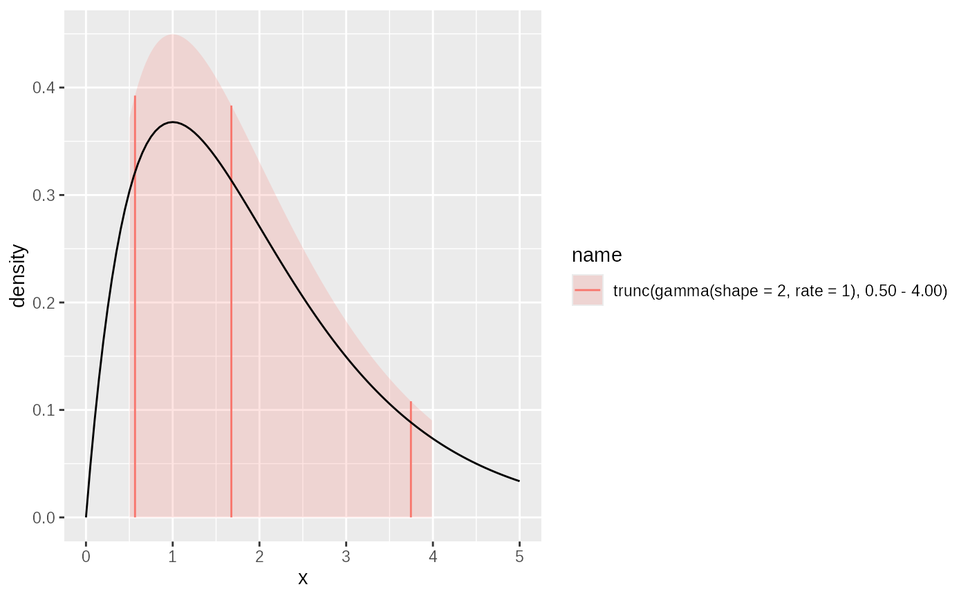
Examples


shape2_gamma = as.dist_fns(pgamma, shape=2)
g2 = truncate(shape2_gamma, 0.5, 4)
plot(g2)+ggplot2::geom_function(fun = ~ dgamma(.x,shape=2), xlim = c(0,5))