Construct a mixture distribution

Constructs a mixture distribution from a list of component distributions \(\text{dist}_i\) with corresponding weights \(w_i\). The CDF \(F_{\text{mix}}\) of the mixture is a weighted sum of the component CDFs: $$ F_{\text{mix}}(x) = \sum_{i=1}^{k} w_i \cdot F_i(x) $$ where \(F_i\) is the CDF of the \(i\)-th component distribution and \(\sum w_i = 1\). The implementation first evaluates the weighted CDF on a grid of \(x\) values (including tail points defined by tail_p and potentially knot points from empirical components). The resulting \((x, F_{\text{mix}}(x))\) pairs are then used as input to empirical_cdf to create the final smooth or piecewise linear dist_fns object representing the mixture distribution.

Usage

mixture(dists, weights = 1, steps = 200, tail_p = 1e-04, ..., name = "mixture")

Arguments

dists

a dist_fn_list of distribution functions

weights

a vector of weights

steps

the number of points that the mixture distribution is evaluated at to construct the empirical mixture

tail_p

the support fo the tail of the distribution

...

Named arguments passed on to empirical_cdf

smooth

fits the empirical distribution with a pair of splines for CDF and quantile function, creating a mostly smooth density. This smoothness comes at the price of potential over-fitting and will produce small differences between p and q functions such that x=p(q(x)) is no longer exactly true. Setting this to false will replace this with a piecewise linear fit that is not smooth in the density, but is exact in forward and reverse transformation.

name

a name for the mixture

Value

a dist_fn of the mixture distribution

Unit tests

dists = c(
  as.dist_fns("norm", mean=-1),
  as.dist_fns("norm", mean=1),
  as.dist_fns("gamma", shape=2)
)
weights = c(1,1,0.3)

mix = mixture(dists,weights)
testthat::expect_equal(
  format(mix),
  "mixture; Median (IQR) 0.289 [-0.886 — 1.31]"
)

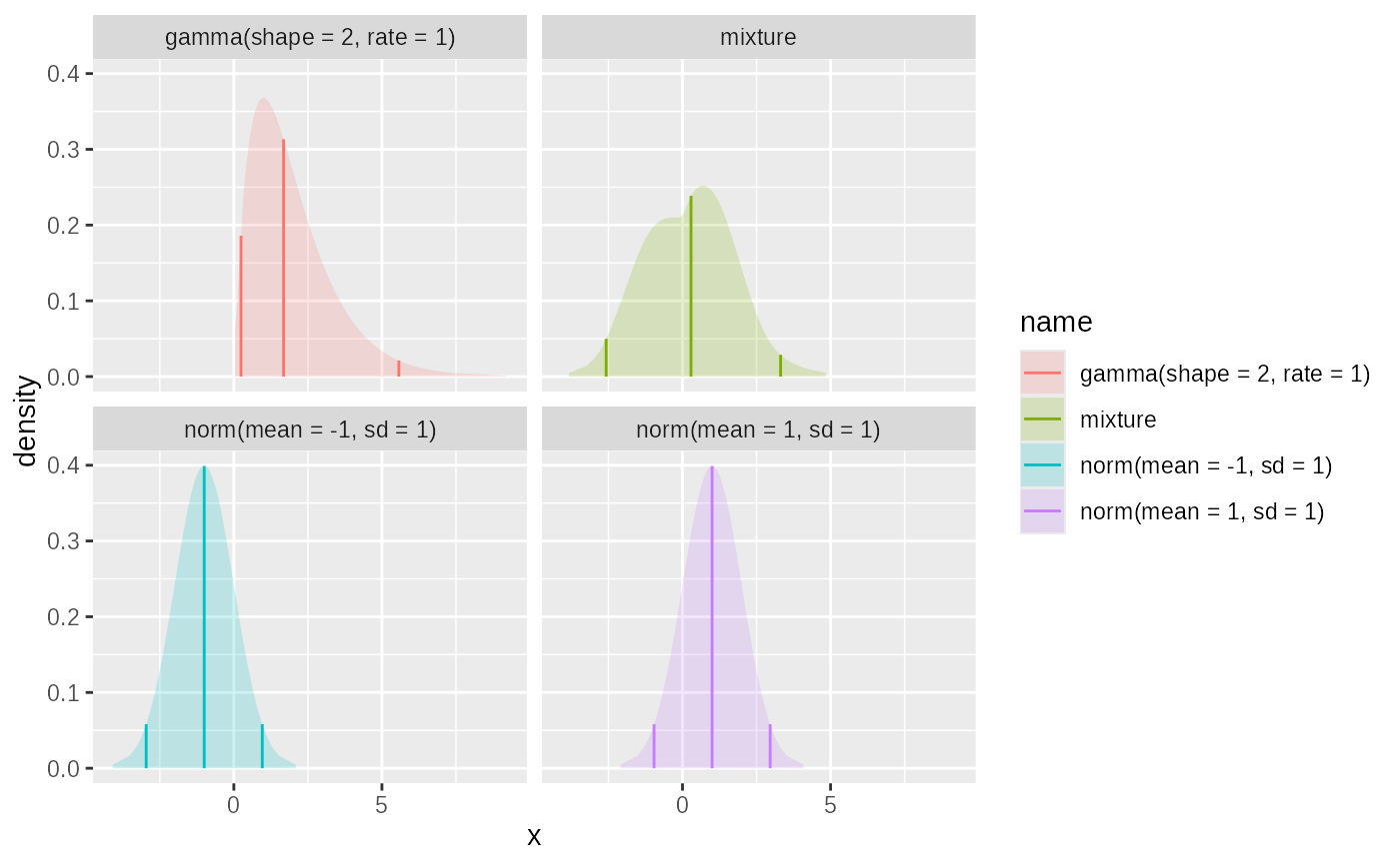
Examples

dists = c(
  as.dist_fns("norm", mean=-1),
  as.dist_fns("norm", mean=1),
  as.dist_fns("gamma", shape=2)
)
weights = c(1,1,0.3)

mix = mixture(dists,weights)
plot(c(dists,mix))+ggplot2::facet_wrap(~name)